Regression Modeling Strategies 4 - Linear Mixed Models
Analyzing Correlated Data Structures in Sports Science
Abstract
Linear mixed models (LMMs) stand as a versatile and robust statistical framework extensively employed in sports science to delve into complex data structures and uncover nuanced relationships among variables. In the realm of sports research, LMMs serve as a cornerstone for analyzing longitudinal or repeated measures data, accounting for both fixed effects—such as player performance or training interventions—and random effects, which encapsulate individual variability or team-specific characteristics. This modeling approach proves particularly adept at handling data with hierarchical or clustered structures, where observations are nested within players, teams, or seasons. Within the sporting domain, LMMs find application in various contexts, including performance analysis, injury prevention, talent identification, and training optimization. For instance, in assessing the effectiveness of training interventions over time, LMMs allow researchers to discern not only the overall impact of a training regimen but also how individual athletes respond differently to the same intervention. Moreover, LMMs enable the exploration of within-subject variability and the identification of factors contributing to fluctuations in performance or injury occurrence across different phases of a season or competition cycle.
Keywords
Mixed models, multilevel models, fixed effects, random effects, repeated measures, hierarchical data, variance components.
Lesson’s Level
The level of this lesson is categorized as SILVER.
Lesson’s Main Idea
- Understanding the importance of correlated data structures and the assumption of independence.
- Constructing linear mixed models with different random effects (e.g., random intercepts, random slopes, and combinations).
- Using fit metrics, such as BIC and AIC, to build a final model.
- Interpreting model parameters, including fixed effects and variance components, from a linear mixed model.
Dataset Used In This Lesson
In this lesson, we use the GovRec dataset from the speedsR package, an R data package specifically designed for the SPEEDS project. This package provides a collection of sports-specific datasets, streamlining access for analysis and research in the sports science context.
1 Introduction: Linear Mixed Models
1.1 Why Linear Mixed Models?
In the previous lessons, we explored regression models that did not violate the assumption of Independence.
Reminder: Independence
The assumption of independence refers to the assumption that the occurrence or outcome of one event is not influenced by the occurrence or outcome of another event. For example, if Team A is playing against Team B in one match and Team X is playing against Team Y in another match, the assumption of independence implies that the result of the Team A vs. Team B match does not influence the result of the Team X vs. Team Y match. Whether Team A wins or loses does not affect the likelihood of Team X winning or losing their match. Each match’s outcome is independent of the other.
Quite often, especially in sport and exercise science, you will encounter situations that violate the assumption of independence. Unfortunately, if we ignore this assumption (and just use our regular linear regression techniques), our estimates may be completely biased and incorrect. This is where the Linear Mixed Model can help.
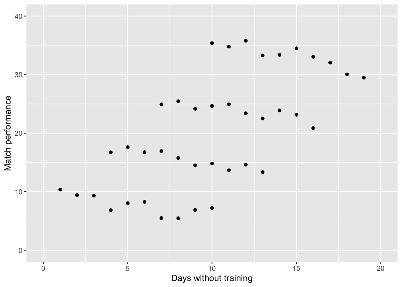
Consider a data set that consists of two variables for 40 different athletes:
Match performance(a continuous variable where higher values represent better performance on the day of an important match)Days without training(the number of days the athlete has missed / skipped training before said match)
Click on the tabs below to explore this scenario and see what happens when Independence is ignored.
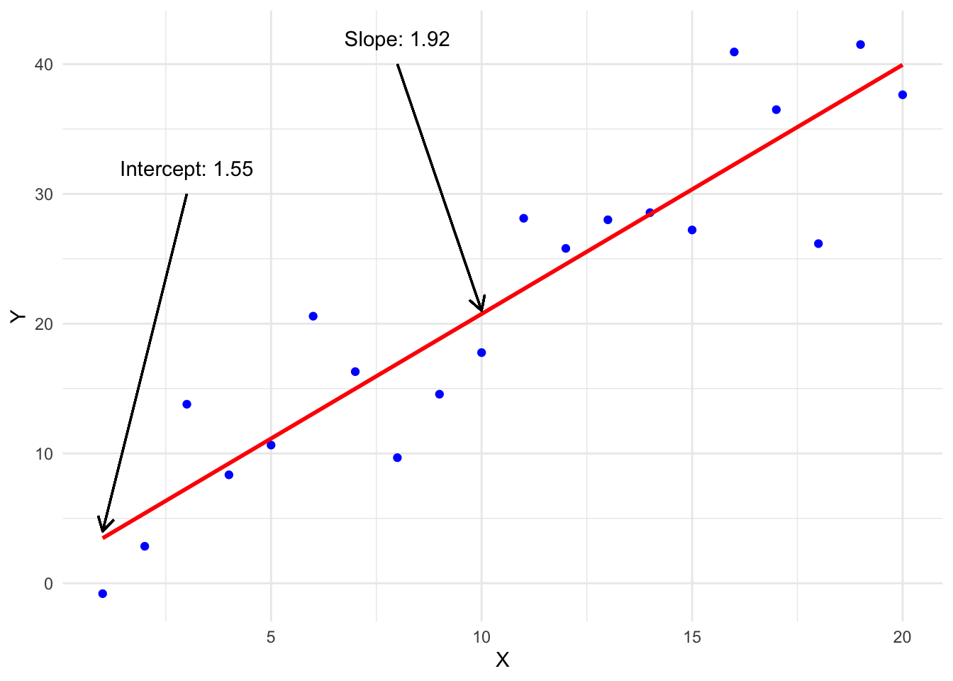
If we were to plot this data, then the graph would illustrate this relationship. Visually, it appears that there is a linear relationship between the two variables (i.e. more days of training missing \(=\) better match performance). This is an odd finding!
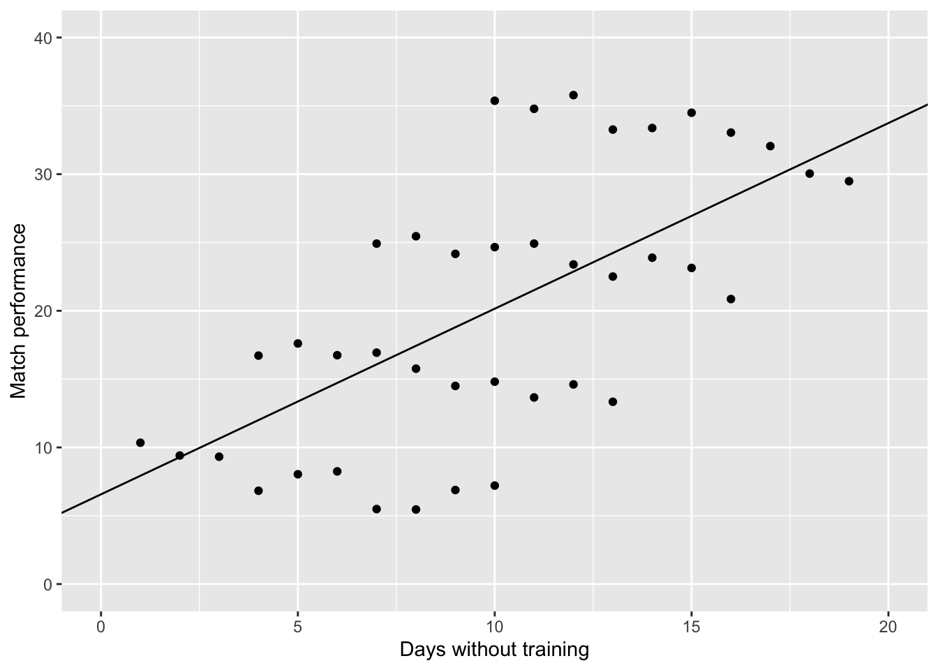
Using Linear Regression, we can add a linear model to this data. This model does indeed confirm what we suspected visually (more days of training missing \(=\) better match performance). Quick Reminder: One of the assumptions of Linear Regression is Independence.
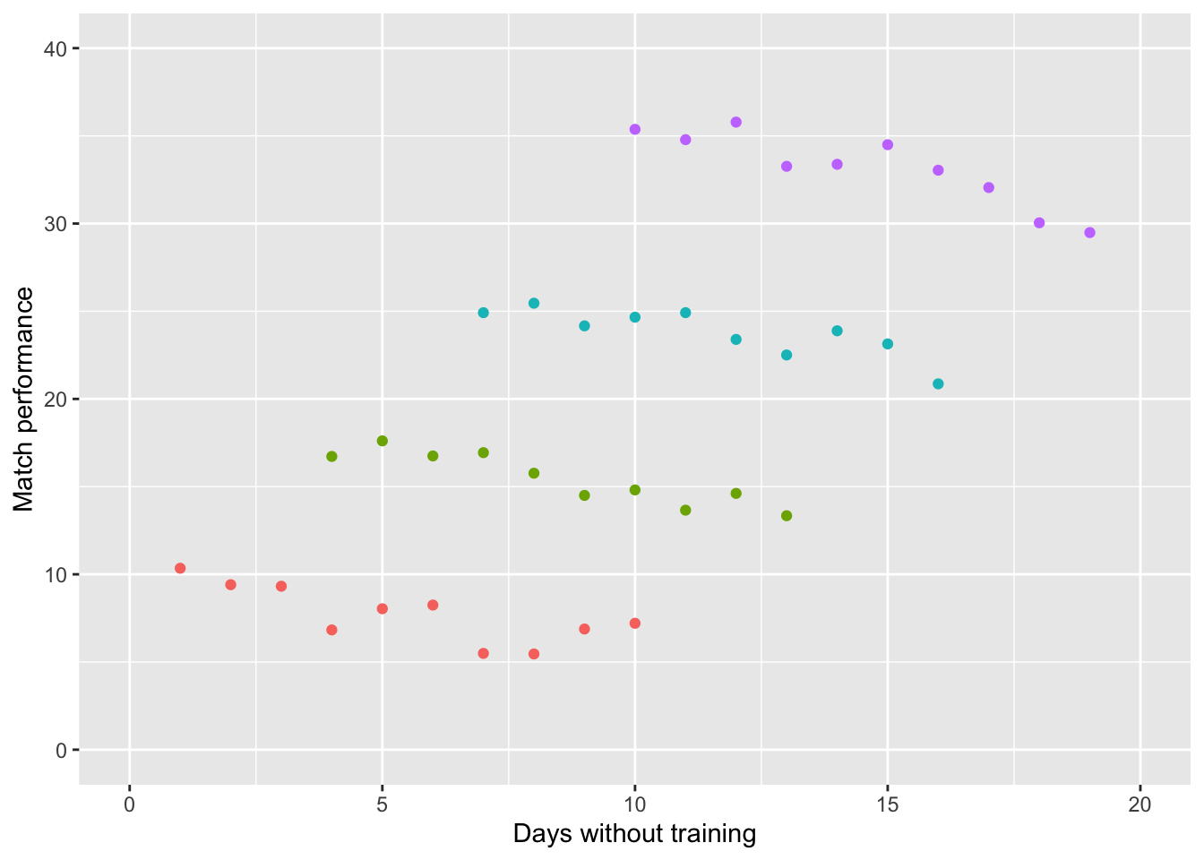
Now assume that each of the 40 athletes belong to 1 of 4 different coaches. Here, I have color coded the coaches to make it easier to distinguish the athletes. Such data violates the assumption of Independence.
If we model the data separately (based on the coach), we can see that there is actually a negative relationship for each of the different models! That is to say:
more days of training missed \(=\) worse performance
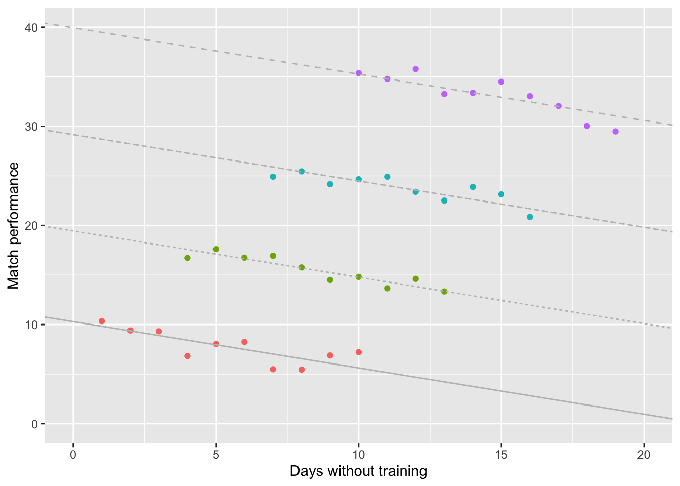
So applying Linear Regression when our data violates Independence (i.e. ignoring the effect of different coaches) would estimate the slope of the overall relationship backwards!
Naturally, this would lead us to interpret the results backwards as well!
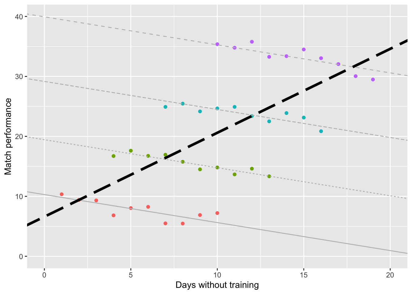
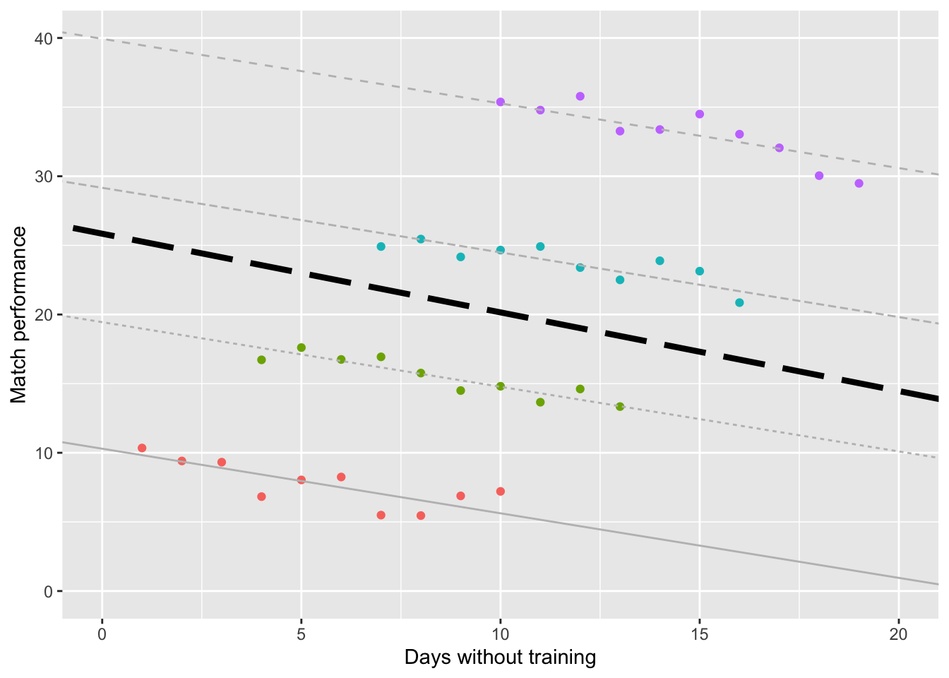
Enter: the Linear Mixed Model (LMM), which can be used when Independence is violated. As we can see from the plot below, the LMM is consistent with the individual models for the 4 coaches.
1.3 Levels
In the context of correlated data structures, such as athletes trained by the same coach or patients treated by the same healthcare provider, the concept of levels refers to the hierarchical structure of the data. Each level represents a different unit of analysis or aggregation within the dataset, with higher levels encompassing lower levels and potentially introducing additional sources of variability or correlation.
For example, consider a study analyzing the performance of athletes within the same sports team. In this scenario, the hierarchical structure may consist of the following levels:
- Level 1 - Individual Athletes: This level represents the lowest level of analysis, with each individual athlete serving as a separate unit of observation. Data collected at this level may include athlete-specific characteristics, such as age, gender, skill level, and performance metrics (e.g., sprint times, jump heights).
- Level 2 - Sports Teams: This level represents the aggregation of individual athletes into sports teams or groups. Data collected at this level may include team-specific variables, such as coaching style, team dynamics, training regimen, and overall team performance.

Within this hierarchical structure, correlations and dependencies may exist both within each level (e.g., similarities among athletes within the same team) and between different levels (e.g., similarities between teams coached by the same coach). Analyzing data at multiple levels allows researchers to account for the nested nature of the data and explore the effects of both individual-level and group-level factors on outcomes of interest.
1.4 Fixed and Random Effects
In statistical modeling, particularly in the context of correlated data structures with hierarchical levels, researchers often need to make decisions about whether to include fixed effects, random effects, or both in their models. Understanding the differences between fixed and random effects is crucial for appropriately modeling the data and drawing accurate conclusions. Let’s delve into each:
1.4.1 Fixed Effects:
Fixed effects are parameters that are treated as constants in the model, representing specific levels or categories of a factor. They are called “fixed” because they are assumed to be fixed and known quantities, rather than being sampled from a larger population.
Characteristics:
- Specific Levels: Fixed effects are used to estimate the effect of specific levels or categories of a factor on the outcome variable.
- Parameter Estimation: In a model with fixed effects, separate coefficients are estimated for each level of the factor.
- Interpretation: The coefficients associated with fixed effects provide information about the average effect of each level of the factor on the outcome variable.
Example: In a study examining the effect of different training programs on sprint performance, fixed effects would estimate the average improvement in sprint times associated with each training program.
1.4.2 Random Effects:
Random effects, on the other hand, are variables that are treated as random draws from a larger population. They represent variability within a particular level of a factor, capturing unobserved heterogeneity or random variation that is shared among observations within the same level.
Characteristics:
- Shared Variability: Random effects capture variability that is shared among observations within the same level of a factor.
- Parameter Estimation: In a model with random effects, parameters are estimated for the distribution of the random effects rather than for each individual level of the factor.
- Interpretation: The variance component associated with random effects quantifies the amount of variability within each level of the factor.
Example: In a study analyzing the effect of coaching style on athlete performance, random effects would capture the variability in performance outcomes that is shared among athletes coached by the same coach.
1.4.3 Fixed vs. Random Effects:
Considerations:
- Interpretation: Fixed effects provide information about the average effect of specific levels of a factor, while random effects capture variability within levels.
- Model Complexity: Including random effects can increase the complexity of the model but may provide a more accurate representation of the data structure.
- Inference: Fixed effects are often used for hypothesis testing and making inferences about specific levels of a factor, while random effects are useful for estimating overall variance and accounting for clustering within levels.
Integration: In many cases, both fixed and random effects may be included in the same model to account for different sources of variability and provide a comprehensive understanding of the data. This approach, known as mixed-effects modeling, allows researchers to simultaneously estimate fixed effects associated with specific factors of interest and random effects associated with variability within levels of those factors.
1.4.4 Slopes & Intercepts
Now that we understand the distinctions between fixed and random effects, let’s delve deeper into the critical decisions surrounding slopes and intercepts when constructing LMMs for correlated data structures. See the textbox below for a reminder on intercepts and slopes.
Reminder: Intercepts & Slopes
Intercept: In statistical modeling, the intercept (often denoted as β0) is a constant term in the model equation that represents the predicted value of the outcome variable when all predictor variables are set to zero. It represents the starting point of the regression line when all predictors have zero values.
Slope: The slope (often denoted as β1) represents the rate of change in the outcome variable for a one-unit change in the predictor variable. It quantifies the strength and direction of the relationship between the predictor and outcome variables.
Click on the tabs below to visualise models with different fixed and random effects for intercepts and slopes:
The data
We will consider the same example from section 1 (athletes clustered within different coaches). In the plot below, each point represents a different athlete. The colors represent different coaches (or clusters). The dependent variable is performance score, and the independent variable is weeks of training missed.

Fixed Intercept & Slope
Fitting an ordinary linear model, with fixed intercept and slope, would ignore the correlated data structure, and assume each athlete has the same starting performance score (intercept), and the same rate of decrease in performance score (slope).

Random Intercepts
It may be the case that each coach has a different starting performance score for their athletes, while the rate at which performance decreases is consistent across all athletes. If we believe this to be the case, we would want to allow the intercept to vary by coach.

Random Slopes
Alternatively, we could imagine that athletes performance starts at the same level (fixed intercept) but decreases at different rates depending on the coach. We could incorporate this idea into a statistical model by allowing the slope to vary, rather than the intercept.

Random Intercepts & Slopes
It’s reasonable to imagine that the most realistic situation is a combination of the scenarios described as: “Athletic performance start at different levels and decrease at different rates depending on the coach.” To incorporate both of these realities into our model, we want both the slope and the intercept to vary.

2 Assumptions
- Linearity: The relationship between the predictors and the response variable is assumed to be linear.
- Normality of residuals: The residuals are assumed to be normally distributed.
- Homogeneity of variances: The variance of the residuals remains constant across all levels of the predictors.
- Normality of random effects: The random effects are assumed to be normally distributed.
3 Case Study
3.1 What to expect
In this lesson we will investigate the impact of recovery methods, such as compression garments and electrical stimulation, on the countermovement jump (CMJ) height of elite cross-country skiers relative to a control group, post competition. Measurements will be conducted at baseline and at 8, 20, 44, and 66 hours after a competition.
Specifically, we will investigate if there is a main effect for TIME and CONDITION, as well as an interaction effect for TIME\(\times\)CONDITION.
3.2 Data Loading and Cleaning
For this exercise, we will use the GovRec dataset from the speedsR package.
# Load the speedsR package
library(speedsR)

# Access and assign the dataset to a variable
Recovery <- GovRec
3.3 Initial Exploratory Analyses
3.3.1 Data organisation
GovRec is a data set that contains 9 variables:
ID: Athlete IDSEX: Male, FemaleTIME: Baseline, 8 hours post-race; 20 hours post-race; 44 hours post-race; 68 hours post-raceCONDITION: Recovery Condition (Control; compression garment; electrical stimulation)CK: Creatine kinase (ukat)UREA: Urea (mmol/L)DP_PEAK: Double pole ergometer test peak power (W)CMJ_HEIGHT: Countermovement jump height (cm)SLEEP_HOURS: Self reported sleep (hours)
To begin, we’re going to clean our data. This will involve converting some of the variables to factors and redefining the levels within TIME and CONDITION so that “Baseline” and “Control” can be used as reference levels.
Recovery_cleaned <- Recovery |>
  as_tibble() |>
  mutate_at(c('ID','SEX'), as.factor) |>
  mutate(TIME = factor(TIME, levels = c('Baseline',
                                        '8 h Post-Race',
                                        '20 h Post-Race',
                                        '44 h Post-Race',
                                        '68 h Post-Race'))) |>
  mutate(CONDITION = factor(CONDITION, levels = c('Control',
                                                  'Compression',
                                                  'Electrical Stimulation')))
Given the known sex differences for urea and CMJ height, we will construct separate models for males and females:
Recovery_cleaned_F <- Recovery_cleaned |> filter(SEX == 'F')
Recovery_cleaned_M <- Recovery_cleaned |> filter(SEX == 'M')
3.3.2 Summary statistics
An initial exploration of CMJ_HEIGHT reveals a somewhat normal distribution, with values primarily between 16cm and 46cm.
ggplot(Recovery_cleaned, aes(CMJ_HEIGHT)) +
  geom_histogram()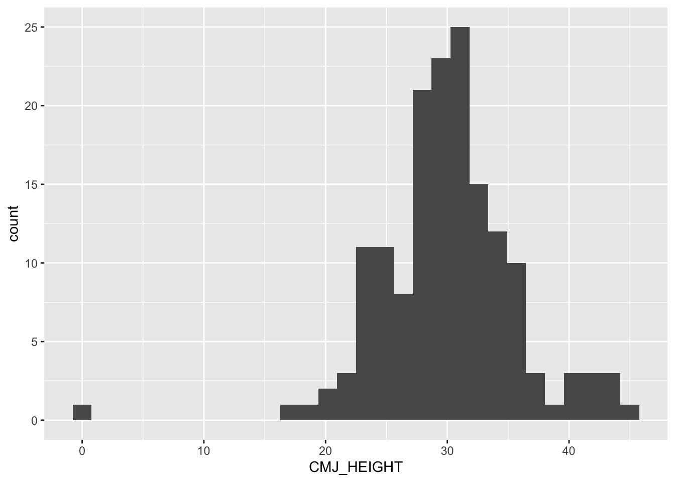
There is an outlier at 0 cm (a male participant), which is implausible based on the context of the measurement. This value will be removed from further analyses to maintain data integrity.
# Filter for full data
Recovery_cleaned <- Recovery_cleaned |> filter(CMJ_HEIGHT > 0)

# Filter for males
Recovery_cleaned_M <- Recovery_cleaned |> filter(SEX == 'M',
                                                 CMJ_HEIGHT > 0)
We can use the skimr package to quicky obtain summary statistics for our chosen variables:
skim_m <- skimr::skim(Recovery_cleaned_M)
skim_f <- skimr::skim(Recovery_cleaned_F)
skim_m |> filter(skim_type == 'factor') |> select(2,6,7)# A tibble: 4 × 3
skim_variable factor.n_unique factor.top_counts
<chr> <int> <chr>
1 ID 18 1: 5, 4: 5, 6: 5, 7: 5
2 SEX 1 M: 87, F: 0
3 TIME 5 Bas: 18, 68 : 18, 8 h: 17, 20 : 17
4 CONDITION 3 Con: 30, Ele: 30, Com: 27 In the output above (for men) we can see that each of the 18 IDs have 5 measurements (Baseline to 68h post competition). As explained in section 1, this is a correlated data structure, where CMJ height measurements will be similar within the same athlete. Thus, we can treat ID as a cluster variable.
3.3.3 Time effects
Next, let us explore how CMJ_HEIGHT changes over time. Given the known biological differences between males and females, we will split the plots by SEX:
# Relabel the time factors so it fits better on the plots
Recovery_cleaned_Time.01 <-
  Recovery_cleaned |>
  mutate(TIME = case_when(
    TIME == 'Baseline' ~ 0,
    TIME == '8 h Post-Race' ~ 1,
    TIME == '20 h Post-Race' ~ 2,
    TIME == '44 h Post-Race' ~ 3,
    TIME == '68 h Post-Race' ~ 4,
  ))

# Create a plot for TIME versus CMJ Height
n1 <- ggplot(Recovery_cleaned_Time.01, aes(TIME, CMJ_HEIGHT)) +
  geom_line(aes(group = ID), color = 'dark grey') +
  geom_smooth(aes(group = 1), color = 'black') +
  facet_wrap(~SEX)

# Same as above but factoring in CONDITION
n2 <- ggplot(Recovery_cleaned_Time.01, aes(TIME, CMJ_HEIGHT, color = CONDITION)) +
  geom_line(aes(group = ID), color = 'dark grey') +
  geom_smooth(aes(group = CONDITION)) +
  theme(legend.position = 'right',
        legend.text = element_text(size = 7),
        legend.title = element_text(size = 7)) +
  facet_wrap(~SEX)

# Place the plots on top of each other
library(patchwork)
n1 / n2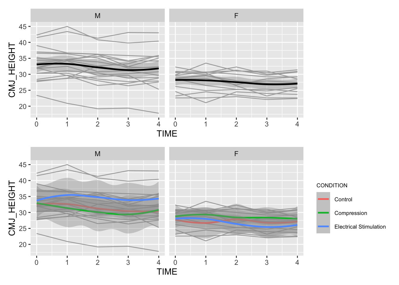
In the plot above, the gray lines represent individual IDs and their change in CMJ_HEIGHT over the 5 time points. The black line (top panel) represents the main effect for time (i.e. when you average all of the individual effects).
- From the top panel, we can see that whilst Males typically have higher
CMJ_HEIGHTScompared the females (as expected), the change over time appears similar for both sexes. - In the bottom panel, we can see how CMJ height changes over time when split by recovery condition. There are some noticeable differences here, so we should take note of these when we run the main analysis.
3.4 Buldining the LMM
3.4.1 An initial model
The first model fit in almost any multilevel context should be the unconditional means model, also called a random intercepts model. In this model, there are no predictors at either level; rather, the purpose of the unconditional means model is to assess the amount of variation at each level—to compare variability within subject to variability between subjects. Expanded models will then attempt to explain sources of between and within subject variability.
# Load libraries
library(lme4)
library(lmerTest)

# Build unconditional means model for females
mod0_F <- lmer(CMJ_HEIGHT ~ 1 + (1|ID), data = Recovery_cleaned_F)

# Build unconditional means model for males
mod0_M <- lmer(CMJ_HEIGHT ~ 1 + (1|ID), data = Recovery_cleaned_M)
Using the summary function, let us examine the random effects in the model (we don’t care about the fixed effects now because we haven’t added any predictors yet)
VCrandom_F <- VarCorr(mod0_F)
print(VCrandom_F, comp = c("Variance", "Std.Dev."))
Groups Name Variance Std.Dev.
ID (Intercept) 8.5842 2.9299
Residual 1.7150 1.3096 From this output:
- \(\sigma^2=1.72\): the estimated variance in within-person deviations.
- \(\sigma^2_u=8.58\): the estimated variance in between-persons deviations.
The relative levels of between- and within-person variabilities can be compared through the intraclass correlation coefficient (ICC):
\[ICC=\frac{Between\space variability}{Total\space variability}=\frac{8.58}{8.58+1.72}=.833\]
Thus, 83.3% of the total variability in CMJ height for females are attributable to differences among subject. Note: as ICC approaches 0, responses from an individual are essentially independent and accounting for the multilevel structure of the data becomes less crucial. However, as ICC approaches 1, repeated observations from the same individual essentially provide no additional information and accounting for the multilevel structure becomes very important.
Repeating this for males:
VCrandom_M <- VarCorr(mod0_M)
print(VCrandom_M, comp = c("Variance", "Std.Dev."))
Groups Name Variance Std.Dev.
ID (Intercept) 26.4708 5.1450
Residual 2.5833 1.6073 Here, the ICC (\(\frac{26.47}{26.47+2.58}=.911\)) tells us that 91.1% the total variability in CMJ height for males are attributable to differences among subject.
Using the plot_model() function from sjPlot, we can visualise this random effects to get a sense of the variability between and within participants. In the function we would specify type = 're' (where re = random effect).
sjPlot::plot_model(mod0_F, type = 're', grid = F, sort.est = T)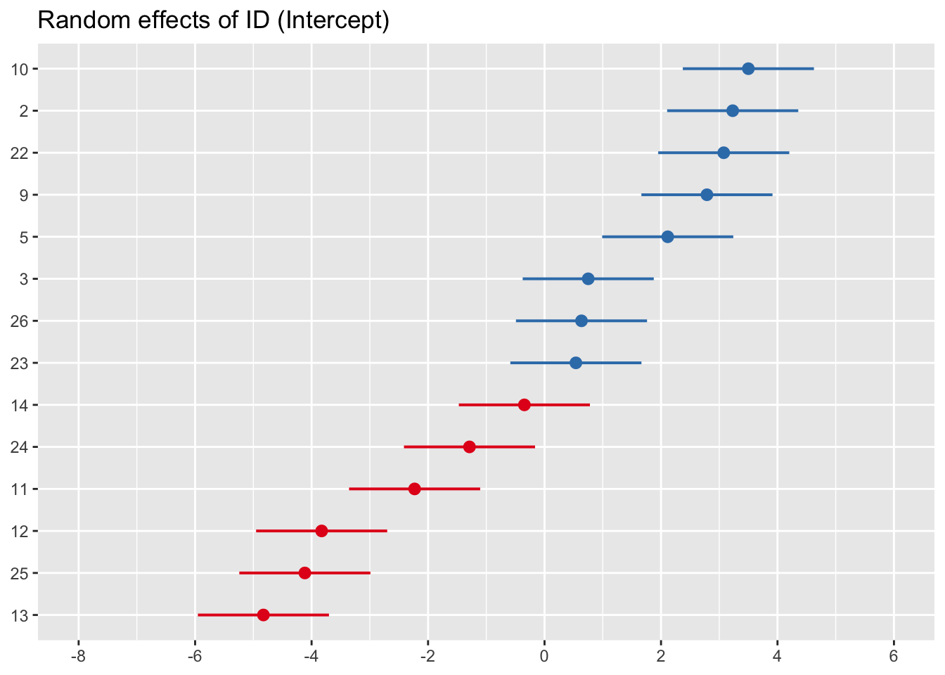
sjPlot::plot_model(mod0_M, type = 're', grid = F, sort.est = T)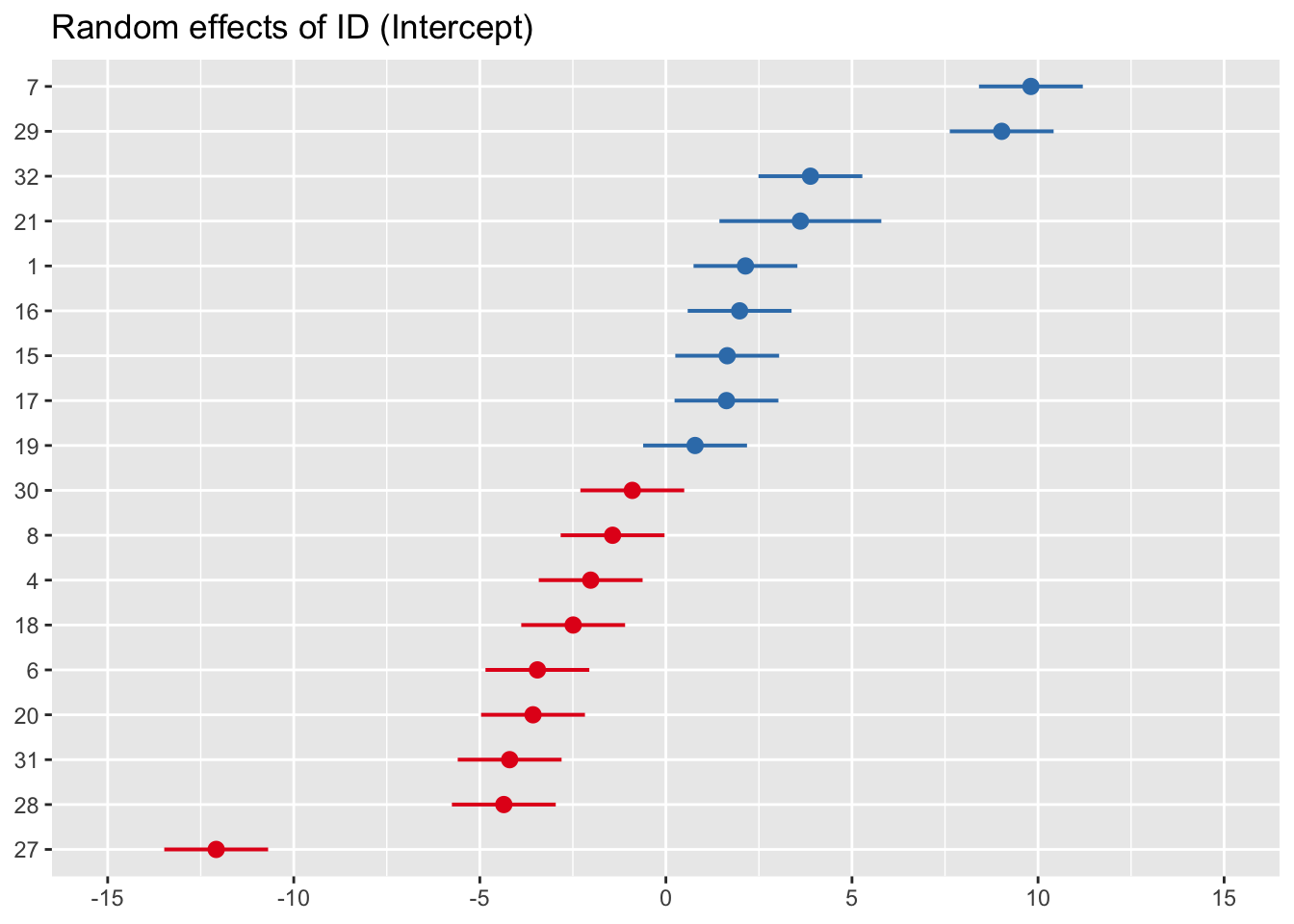
3.4.2 Adding effects
Let us now add in the main and interaction effects to our models:
# Build model for females
mod1_F <- lmer(CMJ_HEIGHT ~ TIME + CONDITION + TIME:CONDITION + (1|ID),
               data = Recovery_cleaned_F)

# Build model for males
mod1_M <- lmer(CMJ_HEIGHT ~ TIME + CONDITION + TIME:CONDITION + (1|ID),
               data = Recovery_cleaned_M)
We can use the anova function to create an analysis of variance table which tests whether the model terms are significant. The function can also be used to compared deviances from different models to assess model fit. In our example, we are using it to see if the interaction time TIME\(\times\)CONDITION is significant. As a reminder (see Lesson 1), our goal with modeling should be to obtain the simplest model possible while retaining its predictive and explanatory power. Thus, removing non-significant interactions identified helps streamline the model’s complexity, ensuring that it remains parsimonious without sacrificing its ability to capture essential relationships between variables.
anova(mod1_F)Type III Analysis of Variance Table with Satterthwaite's method
Sum Sq Mean Sq NumDF DenDF F value Pr(>F)
TIME 18.1087 4.5272 4 44 3.3582 0.0175 *
CONDITION 1.1898 0.5949 2 11 0.4413 0.6541
TIME:CONDITION 16.5989 2.0749 8 44 1.5391 0.1715
---
Signif. codes: 0 '***' 0.001 '**' 0.01 '*' 0.05 '.' 0.1 ' ' 1anova(mod1_M)Type III Analysis of Variance Table with Satterthwaite's method
Sum Sq Mean Sq NumDF DenDF F value Pr(>F)
TIME 45.363 11.3408 4 57.044 5.8839 0.0004911 ***
CONDITION 2.471 1.2356 2 15.007 0.6411 0.5405550
TIME:CONDITION 23.261 2.9077 8 57.042 1.5086 0.1746394
---
Signif. codes: 0 '***' 0.001 '**' 0.01 '*' 0.05 '.' 0.1 ' ' 1In the two outputs above, we can see that the neither interaction effects are statistically significant. Thus, it makes sense to remove them for model simplicity.
Our next models will become:
# Build model for females
mod2_F <- lmer(CMJ_HEIGHT ~ TIME + CONDITION + (1|ID),
               data = Recovery_cleaned_F)

# Build model for males
mod2_M <- lmer(CMJ_HEIGHT ~ TIME + CONDITION + (1|ID),
               data = Recovery_cleaned_M)
We can use the anova function to compare
anova(mod2_F,mod1_F)Data: Recovery_cleaned_F
Models:
mod2_F: CMJ_HEIGHT ~ TIME + CONDITION + (1 | ID)
mod1_F: CMJ_HEIGHT ~ TIME + CONDITION + TIME:CONDITION + (1 | ID)
npar AIC BIC logLik deviance Chisq Df Pr(>Chisq)
mod2_F 9 284.75 304.99 -133.38 266.75
mod1_F 17 286.94 325.16 -126.47 252.94 13.817 8 0.08666 .
---
Signif. codes: 0 '***' 0.001 '**' 0.01 '*' 0.05 '.' 0.1 ' ' 1As a reminder from lesson 1, AIC and BIC are metrics that we can use to assess model fit, with lower values representing better fit. From the output above, model 2 (no interaction effect) fits the data better compared to model 1 (with the time\(\times\)condition effect). A test of the model deviances revealed no significant difference between the two (p = .087). Thus, the simpler method (without the interaction) should be the preferred model.
A similar observation is noted for males as well:
anova(mod2_M,mod1_M)Data: Recovery_cleaned_M
Models:
mod2_M: CMJ_HEIGHT ~ TIME + CONDITION + (1 | ID)
mod1_M: CMJ_HEIGHT ~ TIME + CONDITION + TIME:CONDITION + (1 | ID)
npar AIC BIC logLik deviance Chisq Df Pr(>Chisq)
mod2_M 9 395.03 417.22 -188.51 377.03
mod1_M 17 397.75 439.67 -181.88 363.75 13.278 8 0.1026We can also use the tab_model() function from the sjPlot package to view both the fixed and random effects in a table. The function also computes the ICC for us:
sjPlot::tab_model(mod2_F, mod2_M,
dv.labels = c('CMJ Height Females','CMJ Height Males'))| CMJ Height Females | CMJ Height Males | |||||
|---|---|---|---|---|---|---|
| Predictors | Estimates | CI | p | Estimates | CI | p |
| (Intercept) | 27.91 | 24.73 – 31.08 | <0.001 | 32.05 | 27.69 – 36.42 | <0.001 |
| TIME [8 h Post-Race] | -0.13 | -1.04 – 0.78 | 0.779 | 0.40 | -0.57 – 1.37 | 0.414 |
| TIME [20 h Post-Race] | -0.68 | -1.59 – 0.23 | 0.142 | -0.70 | -1.67 – 0.27 | 0.154 |
| TIME [44 h Post-Race] | -1.36 | -2.27 – -0.44 | 0.004 | -1.53 | -2.50 – -0.56 | 0.002 |
| TIME [68 h Post-Race] | -1.14 | -2.06 – -0.23 | 0.015 | -1.23 | -2.18 – -0.28 | 0.012 |
| CONDITION [Compression] | 1.34 | -2.85 – 5.53 | 0.525 | 0.06 | -6.05 – 6.18 | 0.984 |
| CONDITION [Electrical Stimulation] |
-0.46 | -4.65 – 3.74 | 0.828 | 2.99 | -3.12 – 9.10 | 0.333 |
| Random Effects | ||||||
| σ2 | 1.46 | 2.04 | ||||
| τ00 | 9.47 ID | 27.83 ID | ||||
| ICC | 0.87 | 0.93 | ||||
| N | 14 ID | 18 ID | ||||
| Observations | 70 | 87 | ||||
| Marginal R2 / Conditional R2 | 0.077 / 0.877 | 0.078 / 0.937 | ||||
From the output above we can see that:
For females, CMJ height is 1.36cm lower at 44h post-race compared to baseline (95% CI = -2.27 to -0.44, p = .004); and 1.14cm lower at 68h post-race compared to baseline (95% CI = -2.06 to -0.23, p = 0.015), when controlling for recovery condition. The random effects indicate the average between subject standard deviation in CMJ height to be 1.46cm, with a variability of 9.47cm across individual subjects. The ICC reveals that 87% of the total variability in CMJ height can be attributed to differences among individual subjects.
For males, CMJ height is 1.53m lower at 44h post-race compared to baseline (95% CI = -2.50 to -0.56, p = .002); and 1.23m lower at 68h post-race compared to baseline (95% CI = -2.18 to -0.28, p = 0.012), when controlling for recovery condition. The random effects indicate the average between subject standard deviation in CMJ height to be 2.04cm, with a variability of 27.83cm across individual subjects. The ICC reveals that 93% of the total variability in CMJ height can be attributed to differences among individual subjects.
Note: The interpretation above is only relevant to the Control group, which is the reference level. To interpret for Compression and Electrical stimulation conditions as well, we can add the estimates for each effect of interest together. For example, if we look at the Female model, the estimated mean CMJ height for each of the three conditions at baseline can be calculated by adding the Intercept estimate (27.91) to the estimate for the other two conditions (1.34 and -0.46, respectively):
Baseline:
- Control = 27.91 cm
- Compression = 27.91 + 1.34 = 29.25 cm
- Electrical S. = 27.91 - 0.46 = 27.45 cm
These baseline values can then be added to estimate for each time point from the table to view the mean CMJ height:
8h Post-Race:
- Control = 27.91 - 0.13 = 27.78 cm
- Compression = 27.91 + 1.34 - 0.13 = 29.12 cm
- Electrical S. = 27.91 - 0.46 - 0.13 = 27.32 cm
20h Post-Race:
- Control = 27.91 - 0.68 = 27.23 cm
- Compression = 27.91 + 1.34 - 0.68 = 28.44 cm
- Electrical S. = 27.91 - 0.46 - 0.68 = 26.64 cm
This can then be repeated for the other time points as well
3.4.3 Random Intercepts & Slopes
Now that we have seen how to add random intercepts to a model, the next step is to consider the inclusion of random slopes. While random intercepts account for variations in the baseline level of the response variable across different groups or individuals, random slopes take our modeling capabilities a step further by allowing for the exploration of varying relationships between predictors and the response within these groups. Incorporating random slopes acknowledges that the effect of predictors may not remain constant across different levels of grouping factors. Instead, it acknowledges the possibility that individuals or groups may exhibit distinct trends or patterns in their responses, resulting in variations in the slopes of regression lines.
A common challenge with building a mixed model is determine which of your variables should be fixed, and which should be random (or both fixed and random). In our current example, we had previously fit CONDITION as a fixed effect only. Let us now explore fitting it as a random slope as well:
# Build model for females
mod2_F_slopes <- lmer(CMJ_HEIGHT ~ TIME + CONDITION + (CONDITION|ID),
               data = Recovery_cleaned_F)

# Build model for males
mod2_M_slopes <- lmer(CMJ_HEIGHT ~ TIME + CONDITION + (CONDITION|ID),
               data = Recovery_cleaned_M)
Let us now compare this random intercepts slopes model to our previous random intercepts only model:
anova(mod2_F_slopes, mod2_F)Data: Recovery_cleaned_F
Models:
mod2_F: CMJ_HEIGHT ~ TIME + CONDITION + (1 | ID)
mod2_F_slopes: CMJ_HEIGHT ~ TIME + CONDITION + (CONDITION | ID)
npar AIC BIC logLik deviance Chisq Df Pr(>Chisq)
mod2_F 9 284.75 304.99 -133.38 266.75
mod2_F_slopes 14 292.66 324.14 -132.33 264.66 2.0919 5 0.8363anova(mod2_M_slopes, mod2_M)Data: Recovery_cleaned_M
Models:
mod2_M: CMJ_HEIGHT ~ TIME + CONDITION + (1 | ID)
mod2_M_slopes: CMJ_HEIGHT ~ TIME + CONDITION + (CONDITION | ID)
npar AIC BIC logLik deviance Chisq Df Pr(>Chisq)
mod2_M 9 395.03 417.22 -188.51 377.03
mod2_M_slopes 14 400.78 435.31 -186.39 372.78 4.2447 5 0.5147The output here suggests that adding Recovery Condition as a random slope does not improve model fit for neither females or males. In both instances, the random intercept only model has lower AIC and BIC values. In addition, there is no significant change in the deviances (p = .836 and p = .515, respectively).
Note: In general, we should consider the theory behind the effects first, as this can save us some valuable time in the modelling process. E.g. if there is no scientific reason that Recovery Condition would vary for each ID, then there would be no reason to fit it as a random slope. Suppose there is theoretical sense to include Time as a random slope (with Condition). This can be coded as seen below. For the random effects structure, if you want to allow the slopes associated with TIME to vary across levels of ID, you need to convert TIME to numeric in this context. This is because random slopes are generally used for continuous predictors, allowing for variability in the relationship between TIME and the outcome for different individuals (or ID). When TIMEis numeric in the random effects part, it will allow the model to account for how the effect of TIMEon CMJ_HEIGHT might differ for each ID:
# Build model for females
mod3_F_slopes <- lmer(CMJ_HEIGHT ~ TIME + CONDITION + (CONDITION+as.numeric(TIME)|ID),
               data = Recovery_cleaned_F)

# Build model for males
mod3_M_slopes <- lmer(CMJ_HEIGHT ~ TIME + CONDITION + (CONDITION+as.numeric(TIME)|ID),
               data = Recovery_cleaned_M)
Like before, we can compare these new models using the anova() function:
anova(mod3_F_slopes, mod2_F_slopes)Data: Recovery_cleaned_F
Models:
mod2_F_slopes: CMJ_HEIGHT ~ TIME + CONDITION + (CONDITION | ID)
mod3_F_slopes: CMJ_HEIGHT ~ TIME + CONDITION + (CONDITION + as.numeric(TIME) | ID)
npar AIC BIC logLik deviance Chisq Df Pr(>Chisq)
mod2_F_slopes 14 292.66 324.14 -132.33 264.66
mod3_F_slopes 18 298.23 338.70 -131.12 262.23 2.4278 4 0.6576anova(mod3_M_slopes, mod2_M_slopes)Data: Recovery_cleaned_M
Models:
mod2_M_slopes: CMJ_HEIGHT ~ TIME + CONDITION + (CONDITION | ID)
mod3_M_slopes: CMJ_HEIGHT ~ TIME + CONDITION + (CONDITION + as.numeric(TIME) | ID)
npar AIC BIC logLik deviance Chisq Df Pr(>Chisq)
mod2_M_slopes 14 400.78 435.31 -186.39 372.78
mod3_M_slopes 18 400.00 444.38 -182.00 364.00 8.7851 4 0.0667 .
---
Signif. codes: 0 '***' 0.001 '**' 0.01 '*' 0.05 '.' 0.1 ' ' 13.4.3.1 Heterogeneous Level 1 Variance Structures
In many experimental settings, the assumption of homogeneity of variance across groups may not hold true. This can be particularly relevant when dealing with repeated measures data, where variances may differ based on the conditions or time points being evaluated. To address this issue, we can extend our linear mixed model framework by fitting a model that allows for heterogeneous variances.
In this section, we utilize the gls function from the nlme package to specify a generalized least squares model with a structure that accounts for varying residual variances across different levels of the CONDITION factor over time. The model is formulated as follows:
library(nlme)
mod_hetero <- gls(CMJ_HEIGHT ~ TIME * CONDITION,
                  data = Recovery_cleaned_F,
                  weights = varIdent(form = ~TIME | CONDITION))
The model includes the interaction term between TIME and CONDITION, which allows us to assess how the relationship between TIME and the outcome variable, CMJ_HEIGHT, may vary across different conditions. The weights argument specifies that the variances should be modeled as a function of TIME, with separate variance estimates for each CONDITION.
To visualize the model predictions and better understand the effects, we create a new dataset that includes all combinations of TIME and CONDITION for which we want to predict CMJ_HEIGHT. This is achieved using the expand.grid function:
# Create a new dataset for predictions
new_data <- expand.grid(
  TIME = unique(Recovery_cleaned_F$TIME),
  CONDITION = unique(Recovery_cleaned_F$CONDITION)
)

# Add predictions to the new dataset
new_data$predicted_CMJ_HEIGHT <- predict(mod_hetero, newdata = new_data)
With the predictions calculated, we can create a line plot to visualize how CMJ_HEIGHT varies with TIME for each CONDITION. The following code generates this plot:
# Plot the predictions
ggplot(new_data, aes(x = TIME, y = predicted_CMJ_HEIGHT, color = CONDITION)) +
  geom_line(aes(group = CONDITION)) +
  labs(title = "Predicted CMJ Height by TIME and CONDITION",
       x = "Time",
       y = "Predicted CMJ Height") +
  theme_minimal()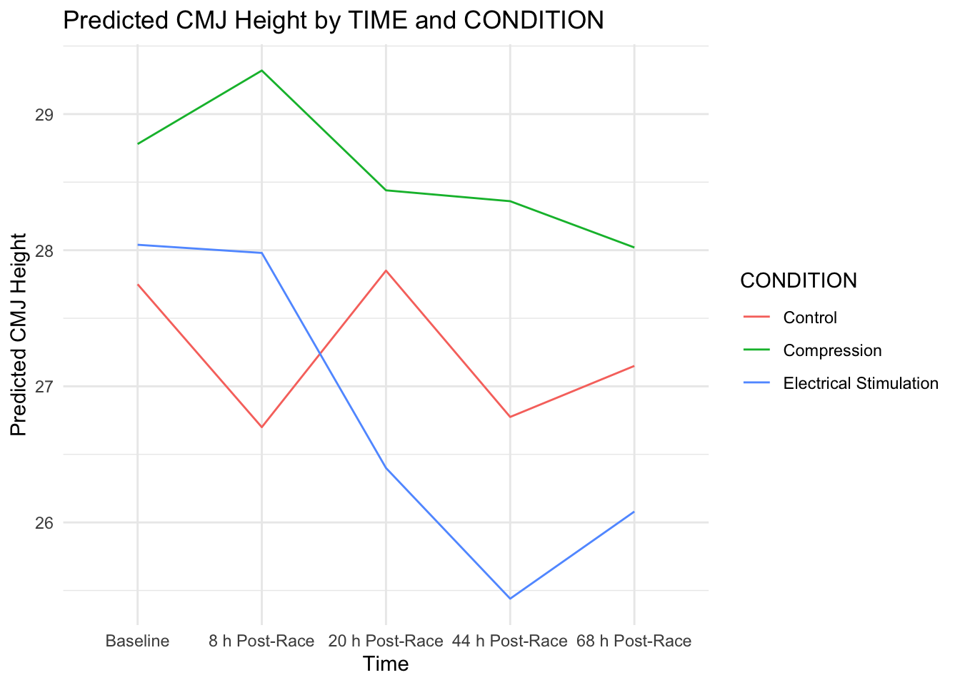
This visualization provides a clear depiction of the predicted relationships, allowing us to observe how the expected CMJ_HEIGHT differs across conditions over time. Such insights are crucial for understanding the dynamics of the data and informing further analyses or interventions. By fitting a model that accounts for heterogeneous variances, we enhance the robustness and interpretability of our findings, ensuring that we appropriately model the complexities inherent in our data.
3.4.4 Checking assumptions
As we have done in previous lessons, we can use the check_model() function from the ‘performance’ package to check the assumptions of the models:
library(performance)
check_model(mod2_F,
            check = c('linearity','homogeneity','qq','reqq','vif','outliers'))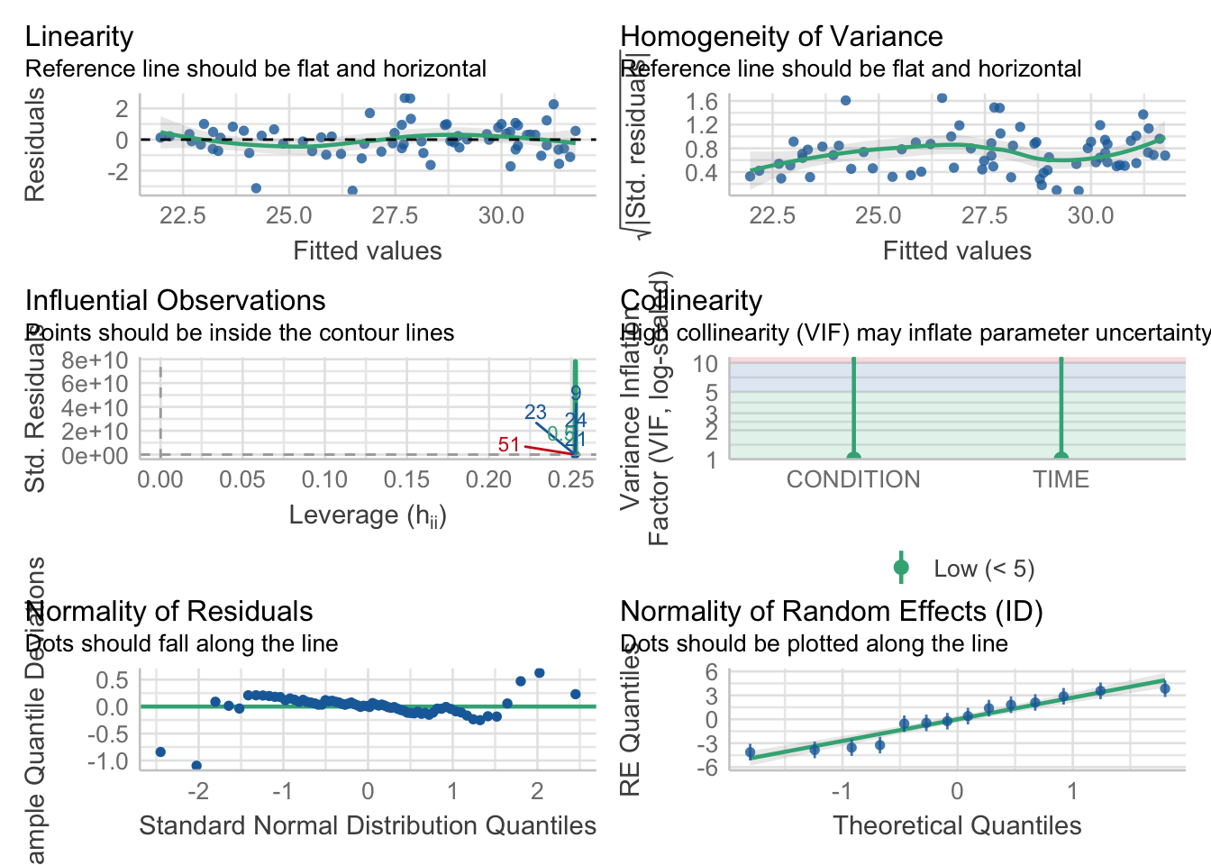
check_model(mod2_M,
            check = c('linearity','homogeneity','qq','reqq','vif','outliers'))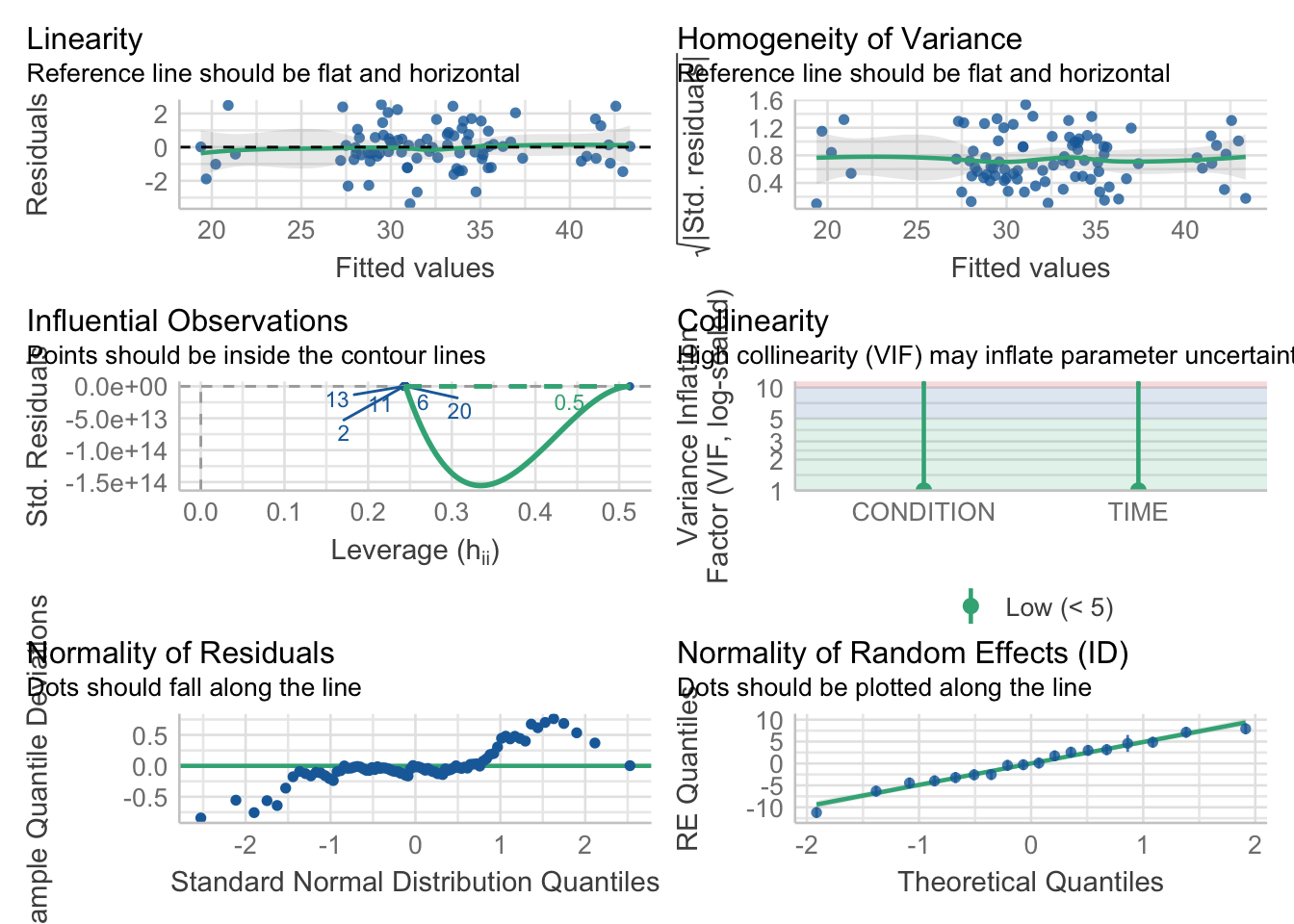
For both models, whilst there is some variation, the assumptions are relatively satisfied, and we can be happy to proceed.
mod9_F <- lmer(CMJ_HEIGHT ~ UREA:CONDITION + (1|ID),
               data = Recovery_cleaned_F)
4 Additional considerations
4.1 Equivalence Testing
Thus far, we have examined this problem under the framework of traditional hypothesis testing, where the focus is on detecting differences between groups or conditions. However, an alternative approach known as equivalence testing offers a different perspective, emphasising the assessment of similarity rather than difference.
In equivalence testing, researchers define a region of practical equivalence (ROPE), representing the range within which the observed difference between treatments is deemed practically indistinguishable. This ROPE is determined based on factors such as clinical relevance, prior knowledge, or regulatory requirements.
Continuing with our example comparing the effectiveness of three recovery methods: control, compression, and electrical stimulation, we could employ equivalence testing to ascertain whether the outcomes produced by these methods are essentially similar.
- Within equivalence testing, two-sided testing assesses whether the observed difference falls entirely within the predefined ROPE. If so, it indicates that the treatments are practically equivalent. Conversely, if the observed difference lies entirely outside the ROPE, it suggests that the treatments are not equivalent within the specified margin. In our scenario, two-sided equivalence testing could be employed to evaluate whether the recovery outcomes associated with compression and electrical stimulation methods are practically equivalent to those of the control method within a predetermined range.
- Alternatively, one-sided testing can focus on determining whether the observed difference exceeds or falls short of the predefined margin, depending on the direction specified in the hypothesis. For instance, if we hypothesise that the compression method is expected to yield recovery outcomes superior to those of the control method, one-sided equivalence testing could be used to assess whether the outcomes produced by compression are practically equivalent to or better than those of the control method.
We can use the equivalence_test() function from the parameters package to test this:
# Female Model from earlier
mod2_F <- lmer(CMJ_HEIGHT ~ TIME + CONDITION + (1|ID),
               data = Recovery_cleaned_F)

# Equivalence test
parameters::equivalence_test(mod2_F,
                             range = 'default')
# TOST-test for Practical Equivalence
ROPE: [-0.31 0.31]
Parameter | 90% CI | SGPV | Equivalence | p
-----------------------------------------------------------------------------------
(Intercept) | [25.25, 30.56] | < .001 | Rejected | > .999
TIME [8 h Post-Race] | [-0.89, 0.63] | 0.410 | Undecided | 0.512
TIME [20 h Post-Race] | [-1.44, 0.08] | 0.260 | Undecided | 0.804
TIME [44 h Post-Race] | [-2.12, -0.59] | < .001 | Rejected | 0.987
TIME [68 h Post-Race] | [-1.91, -0.38] | < .001 | Rejected | 0.964
CONDITION [Compression] | [-2.16, 4.84] | 0.089 | Undecided | 0.904
CONDITION [Electrical Stimulation] | [-3.96, 3.04] | 0.089 | Undecided | 0.885 In the above output, we can see that the ROPE is computed as [-0.31 to 0.31]. This means that the equivalence testing procedure will consider treatment effects to be practically equivalent if the difference falls entirely within this range.
Next, we can examine the confidence intervals (CI) to assess whether the observed differences between treatments fall within the ROPE. The CI provides a range of plausible values for the true treatment effect, and if this range is entirely contained within the ROPE, it suggests that the treatments can be considered equivalent. Conversely, if the CI extends beyond the boundaries of the ROPE, it indicates that the treatments are not equivalent within the specified margin.
The SGPV (Significant Group Probability Value) column provides information about whether the observed difference between treatments is statistically significant. If the SGPV is less than the conventional significance level (typically 0.05), it suggests that the observed difference is statistically significant, indicating that the treatments have different effects. Conversely, if the SGPV is greater than the significance level, it indicates that the observed difference is not statistically significant, suggesting that the treatments may have similar effects.
The Equivalence column indicates whether the observed difference between treatments falls within the region of practical equivalence (ROPE). If the observed difference is entirely contained within the ROPE, it is considered practically equivalent, and the Equivalence column will indicate “Accepted.” On the other hand, if the observed difference extends beyond the boundaries of the ROPE, it is not considered practically equivalent, and the Equivalence column will indicate “Rejected.”
We can create a plot of this to interpret the results better:
parameters::equivalence_test(mod2_F,
                             range = 'default') |>
  plot()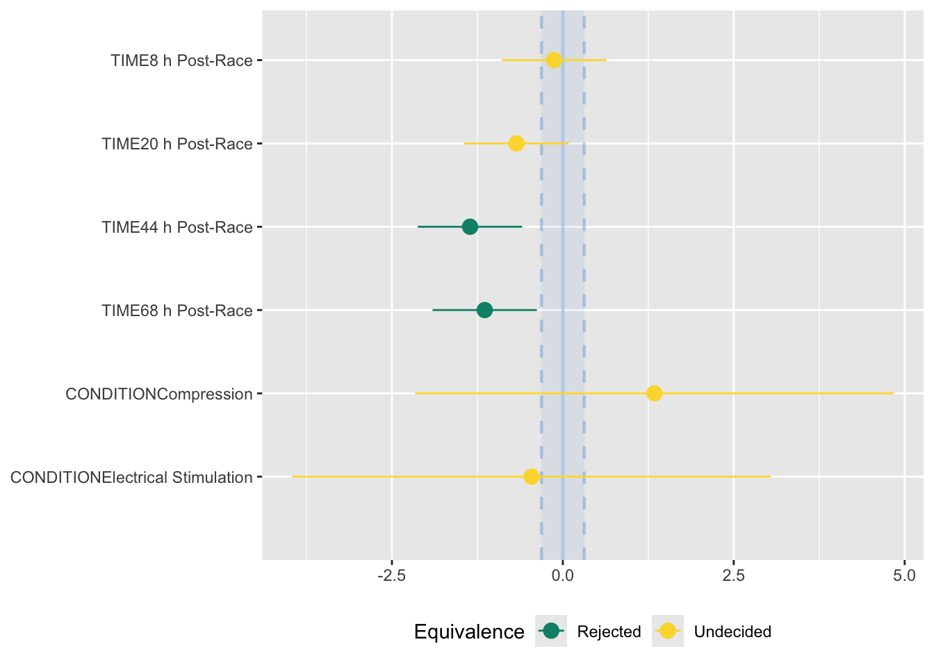
4.2 Modeling Heteroscedasticity
Addressing heteroscedasticity is a crucial aspect to ensure the robustness and validity of our analyses. Heteroscedasticity occurs when the variance of the dependent variable differs across levels of one or more independent variables. This phenomenon challenges the assumption of homogeneity of variance, which assumes that the variability of data points remains constant across all levels of categorical predictors. In our current example, the variability in CMJ heights may differ between recovery methods due to factors such as individual differences, treatment efficacy, or measurement error. To assess this, we can explicitly model and account for heteroscedasticity.
One common approach to address heteroscedasticity in linear mixed-effects models is by specifying a variance structure that allows for different variances between levels of a categorical predictor. In R, this can be achieved using the weights argument in the lme() function from the nlme package.
library(nlme)

# Fit the initial model without considering heteroscedasticity
model0 <- lme(CMJ_HEIGHT ~ TIME + CONDITION,
                    random = ~ 1 | ID,
                    data = Recovery_cleaned_F)

# Fit the model with a variance structure to account for heteroscedasticity
model1 <- lme(CMJ_HEIGHT ~ TIME + CONDITION,
                   random = ~ 1 | ID,
                   weights = varIdent(form = ~ 1 | CONDITION),
                   data = Recovery_cleaned_F)
Next, we can inspect the variance structure of model1 via the summary function:
summary(model1)Linear mixed-effects model fit by REML
Data: Recovery_cleaned_F
AIC BIC logLik
280.1444 303.7188 -129.0722
Random effects:
Formula: ~1 | ID
(Intercept) Residual
StdDev: 3.083958 1.06056
Variance function:
Structure: Different standard deviations per stratum
Formula: ~1 | CONDITION
Parameter estimates:
Control Compression Electrical Stimulation
1.000000 1.035479 1.331279
Fixed effects: CMJ_HEIGHT ~ TIME + CONDITION
Value Std.Error DF t-value p-value
(Intercept) 27.808034 1.5850209 52 17.544270 0.0000
TIME8 h Post-Race -0.161185 0.4425837 52 -0.364192 0.7172
TIME20 h Post-Race -0.506098 0.4425837 52 -1.143509 0.2581
TIME44 h Post-Race -1.148830 0.4425837 52 -2.595734 0.0122
TIME68 h Post-Race -0.999056 0.4425837 52 -2.257328 0.0282
CONDITIONCompression 1.339000 2.0938814 11 0.639482 0.5356
CONDITIONElectrical Stimulation -0.457000 2.1013894 11 -0.217475 0.8318
Correlation:
(Intr) TIME8hP TIME2hP TIME4hP TIME6hP CONDIT
TIME8 h Post-Race -0.140
TIME20 h Post-Race -0.140 0.500
TIME44 h Post-Race -0.140 0.500 0.500
TIME68 h Post-Race -0.140 0.500 0.500 0.500
CONDITIONCompression -0.733 0.000 0.000 0.000 0.000
CONDITIONElectrical Stimulation -0.731 0.000 0.000 0.000 0.000 0.553
Standardized Within-Group Residuals:
Min Q1 Med Q3 Max
-2.7971395157 -0.4754178554 0.0009398415 0.5010172659 2.1781102192
Number of Observations: 70
Number of Groups: 14 The Variance function part of the output indicates the estimated variance parameters associated with each level of the CONDITION variable.
In this output:
- Control (CON) condition: Estimated variance parameter = 1.000000
- Compression (COMP) condition: Estimated variance parameter = 1.035479
- Electrical Stimulation (NMES) condition: Estimated variance parameter = 1.331279
These estimated variance parameters represent the standard deviations of the residuals for each level of the condition variable. Since these values are different for each condition, it suggests the presence of heteroscedasticity (note: conducting an anova() of the two models, or computing confidence intervals can provide further support of the differences in variances between conditions).
4.3 Correlation Structures
In linear mixed models, the correlation structure refers to the pattern of correlation among repeated measurements or observations within the same subject or cluster. This structure captures the dependence between observations and is essential for modeling the covariance matrix of the random effects and residuals accurately. Different correlation structures are available to accommodate various types of data and assumptions about the correlation pattern.
- The default (and what our models have assumed thus far) is the compound symmetric (CS) or exchangeable structure, which assumes that all observations within the same cluster or subject have the same correlation. This structure is appropriate when the correlation between any pair of observations is constant and does not depend on their relative positions.
- Another common correlation structure, especially with repeated measures, is the autoregressive (AR) structure, which assumes that the correlation between observations decreases as the time or distance between them increases. The
corAR1()structure, for example, models the correlation between consecutive observations using a single parameter, often denoted as ρ (rho), representing the autocorrelation coefficient.
As an example, let us use the correlation() function from the nlme package to explore this:
# Fit a model with default correlation structure
model_CS <- lme(CMJ_HEIGHT ~ TIME + CONDITION,
              random = ~ 1 | ID,
              correlation = corCompSymm(),
              data = Recovery_cleaned_F)

# Fit the model with an AR correlation structure
model_AR <- lme(CMJ_HEIGHT ~ TIME + CONDITION,
              random = ~ 1 | ID,
              correlation = corAR1(),
              data = Recovery_cleaned_F)
# Compare models
sjPlot::tab_model(model_CS, model_AR,
dv.labels = c('CS structure','AR structure'))| CS structure | AR structure | |||||
|---|---|---|---|---|---|---|
| Predictors | Estimates | CI | p | Estimates | CI | p |
| (Intercept) | 27.91 | 24.72 – 31.10 | <0.001 | 27.93 | 24.75 – 31.10 | <0.001 |
| TIME [8 h Post-Race] | -0.13 | -1.04 – 0.79 | 0.779 | -0.13 | -0.95 – 0.69 | 0.754 |
| TIME [20 h Post-Race] | -0.68 | -1.59 – 0.24 | 0.143 | -0.68 | -1.62 – 0.27 | 0.156 |
| TIME [44 h Post-Race] | -1.36 | -2.27 – -0.44 | 0.004 | -1.36 | -2.34 – -0.37 | 0.008 |
| TIME [68 h Post-Race] | -1.14 | -2.06 – -0.23 | 0.016 | -1.14 | -2.14 – -0.15 | 0.025 |
| CONDITION [Compression] | 1.34 | -3.28 – 5.95 | 0.536 | 1.27 | -3.32 – 5.87 | 0.554 |
| CONDITION [Electrical Stimulation] |
-0.46 | -5.07 – 4.16 | 0.831 | -0.45 | -5.04 – 4.15 | 0.835 |
| Random Effects | ||||||
| σ2 | 1.46 | 1.75 | ||||
| τ00 | 9.47 ID | 9.11 ID | ||||
| N | 14 ID | 14 ID | ||||
| Observations | 70 | 70 | ||||
| Marginal R2 / Conditional R2 | 0.386 / NA | 0.331 / NA | ||||
The results obtained from these two models, despite utilizing different correlation structures, suggests that either correlation structure might be suitable for analyzing the given dataset. In this instance, both the compound symmetric (CS) and autoregressive (AR) correlation structures produced fixed and random effects.
However, it’s essential to recognize that this may not always be the case. In many scenarios, the choice of correlation structure can significantly impact the model’s results. Depending on the nature of the data and the underlying correlation pattern, different correlation structures may provide more accurate and reliable estimates. For instance, in longitudinal or time-series data where observations are inherently correlated over time, an autoregressive (AR) or moving average (MA) correlation structure may better capture the temporal dependencies between observations. On the other hand, in clustered or grouped data where observations within the same group are correlated, a compound symmetric (CS) or unstructured (UN) correlation structure may be more appropriate.
4.3.1 Evaluating Autocorrelation in Time Series Designs
In time series data, it is crucial to evaluate the autocorrelation structure of the residuals to ensure that the chosen model adequately captures the underlying dependencies in the data. The nlme package can be used to specify the model, and the acf function from the stats package can help us evaluate.
library(nlme)
library(stats)

# Fit the mixed-effects model
model <- lme(CMJ_HEIGHT ~ CONDITION + TIME,
             random = ~ 1 | ID,
             correlation = corAR1(form = ~ as.numeric(TIME) | ID),
             data = Recovery_cleaned_F)

# Extract residuals
residuals_model <- residuals(model, type = "normalized")

# Plot the autocorrelation function
acf(residuals_model, main = "ACF of Model Residuals")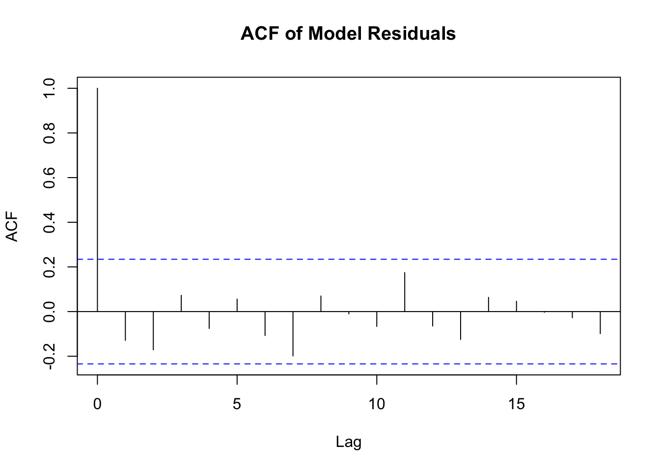
From this plot we can see that autocorrelations at non-zero lags are within the confidence interval (blue dotted lines), suggesting that the AR(1) structure has effectively reduced the temporal correlation in the residuals.
5 Conclusion & Reflection
In conclusion, this guide has provided an overview of linear mixed models, beginning with a vignette for the importance of not violating Independence. We then learnt about correlated data structures, as well as exploring the difference between fixed and random intercepts / slopes. We then learnt how to fit different types of models to our Recovery data.
In addition to their versatility in handling correlated data structures, linear mixed models (LMMs) offer a significant advantage over regular linear models (LMs) by accommodating various types of data distributions and complexities. Unlike LMs, which assume independent observations, LMMs can effectively model correlated data, making them more robust and reliable in real-world applications. Moreover, the concepts learned in Lesson 2 on Poisson regression and Lesson 3 on Logistic Regression extend to generalized linear mixed models (GLMMs), providing a comprehensive toolkit for analyzing correlated data across different scenarios. Understanding the principles of GLMMs opens avenues for exploring more sophisticated statistical techniques in future lessons, enriching our understanding and application of advanced modeling approaches.
Given the inherently multifaceted nature of data collected in sport and exercise science, ranging from athlete performance metrics to physiological responses, the ability to account for correlated structures is paramount. LMMs and GLMMs enable researchers and practitioners to analyze complex datasets while appropriately addressing dependencies, thereby yielding more accurate insights into athlete performance, injury prevention, training optimization, and other critical aspects of sports science. As such, mastering these techniques not only enhances the statistical rigor of analyses but also empowers professionals in sport and exercise science to make informed decisions and drive advancements in athletic performance and well-being.
6 Knowledge Spot Check
How does the assumption of independence differ between linear regression and linear mixed models?
- Linear regression assumes independence of observations within and across groups, while linear mixed models allow for correlated observations within groups.
- Linear regression assumes correlated observations within groups, while linear mixed models assume independence within and across groups.
- Both linear regression and linear mixed models assume independence of observations within and across groups.
- Neither linear regression nor linear mixed models make assumptions about the independence of observations.
- Linear regression assumes independence of observations within and across groups, while linear mixed models allow for correlated observations within groups.
Linear regression assumes that observations are independent of each other, both within and across groups. In contrast, linear mixed models relax this assumption and allow for correlated observations within groups (e.g., repeated measurements on the same individual or clustered data). This flexibility makes linear mixed models suitable for analyzing data with correlated observations, which often occur in longitudinal or clustered study designs.
How does interpreting random effects in linear mixed models differ from interpreting fixed effects?
- Random effects capture systematic variation across groups, while fixed effects capture random variation within groups.
- Random effects represent unobserved, underlying group-level characteristics, while fixed effects represent observed, fixed characteristics.
- Random effects are estimated from the data, while fixed effects are predetermined by the researcher.
- Random effects are interpreted in terms of their effect on the outcome variable’s mean, while fixed effects are interpreted in terms of their effect on the outcome variable’s variability.
- Random effects represent unobserved, underlying group-level characteristics, while fixed effects represent observed, fixed characteristics.
Random effects in linear mixed models capture variation across groups that are not of primary interest but are assumed to be random samples from a larger population of groups. They represent unobserved, underlying group-level characteristics that contribute to the variability in the outcome. In contrast, fixed effects represent observed, fixed characteristics that are of primary interest and are directly estimated from the data.
What term in linear mixed models corresponds to the intercept term in linear regression?
- Random effect
- Fixed effect
- Residual
- Level
- Random effect
In linear mixed models, the random effect term corresponds to the intercept term in linear regression. It captures the variability in the outcome that is not explained by the fixed effects and represents the baseline level of the outcome when all predictor variables are set to zero.
In a linear mixed model analyzing the effect of a training program on athletes’ sprint performance over time, which statement best describes the interpretation of the random slope term (Time|Athlete)?
- The random slope term represents the overall trend of sprint performance improvement across all athletes.
- The random slope term represents the variability in sprint performance improvement among athletes after accounting for the training program.
- The random slope term captures the individual differences in the rate of sprint performance improvement over time for each athlete, accounting for the correlation between repeated measurements from the same athlete.
- The random slope term indicates the average rate of sprint performance improvement across all athletes.
- The random slope term captures the individual differences in the rate of sprint performance improvement over time for each athlete, accounting for the correlation between repeated measurements from the same athlete.
In the context of a linear mixed model analyzing athletes’ sprint performance over time, the random slope term (Time|Athlete) allows for individual variation in the rate of improvement (slope) of sprint performance over time (Time) among different athletes. This term captures how each athlete’s sprint performance changes over time relative to the overall trend, accounting for the correlation between repeated measurements from the same athlete. It does not represent the overall trend of sprint performance improvement or the average improvement rate across all athletes but rather accounts for the variability in improvement trajectories among individual athletes.
Within the context of Linear Mixed Models (LMM), what is the primary purpose of the Intraclass Correlation Coefficient (ICC)?
- Assessing the association between two continuous variables
- Evaluating the reliability or consistency of measurements taken on the same individuals or units across multiple occasions or raters
- Testing the difference in means between two independent groups
- Assessing the goodness of fit of a regression model
- Evaluating the reliability or consistency of measurements taken on the same individuals or units across multiple occasions or raters
In Linear Mixed Models (LMM), the Intraclass Correlation Coefficient (ICC) is commonly used to assess the reliability or consistency of measurements taken on the same individuals or units across multiple occasions or raters. It quantifies the degree of agreement or consistency between measurements, which is essential for ensuring the validity and reproducibility of study findings within the framework of LMMs.