Hbmass <- speedsR::HbmassSynthRegression Modeling Strategies 1 - Linear Regression
Building Foundational Knowledge in Linear Regression Analysis
Abstract
Linear regression is a statistical modeling technique widely employed in sport science to analyze and understand the relationship between two or more variables. In the context of sports, it serves as a valuable tool for examining how changes in one factor, such as training intensity or player performance, correspond to changes in another, such as injury rates or game outcomes. The essence of linear regression lies in fitting a straight line to the data points, allowing researchers and coaches to make predictions and draw insights from the observed patterns. For instance, in sports performance analysis, linear regression might be utilized to assess the impact of various training variables on an athlete’s speed, strength, or endurance. By uncovering these quantitative relationships, sports scientists can optimize training programs, enhance player development strategies, and ultimately contribute to improved athletic performance and well-being.
Keywords
Linear regression, assumptions checking, NHST, simple linear regression, multiple linear regression, residual diagnostics, R, speedsR package, HbmassSynth dataset, predictive modeling, statistical analysis, variance explained, confidence intervals, prediction intervals.
Lesson’s Level
The level of this lesson is categorized as BRONZE.
Lesson’s Main Idea
- Understanding when and how to apply linear regression models effectively in data analysis.
- Developing the ability to evaluate and validate the assumptions underlying linear regression models.
- Leveraging linear regression to interpret relationships between variables in sports science contexts.
Dataset Used In This Lesson
In this lesson, we use the HbmassSynth dataset from the speedsR package, an R data package specifically designed for the SPEEDS project. This package provides a collection of sports-specific datasets, streamlining access for analysis and research in the sports science context. The HbmassSynth dataset offers valuable insights into the effects of moderate altitude exposure and iron supplementation on hematological variables in endurance athletes.
1 Learning Outcomes
By the end of this lesson, you will have developed the ability to:
Construct Linear Regression Models: Build simple and multiple linear regression models in R, applying these techniques to analyze real-world sports science data.
Evaluate Model Assumptions: Use residual diagnostics to examine the assumptions of linear regression models, ensuring model reliability and validity.
Interpret Regression Outputs: Interpret the parameters, confidence intervals, and significance tests from linear regression models to draw meaningful insights about the relationships between variables.
Apply Regression in R: Utilize the
HbmassSynthdataset in thespeedsRpackage to gain hands-on experience in implementing regression modeling techniques.
2 Introduction: Linear Regression
Linear regression is a versatile and widely applied statistical methodology that seeks to model the relationship between a dependent variable (Y) and one or more independent variables (X) by fitting a linear equation to observed data. The technique is suitable when the dependent variable is a continuous outcome, e.g. counter-movement jump height (cm).
The fundamental form of the linear regression equation for a simple linear regression model is represented as \(Y=\beta_{0}+\beta_{1}X+\epsilon\), where \(\beta_{0}\) is the intercept, \(\beta_{1}\) is the slope, \(X\) is the independent variable, and \(\epsilon\) denotes the error terms accounting for unobserved factors. The objective of linear regression is to estimate the coefficients (\(\beta_{0}\) and \(\beta_{1}\)) that minimize the sum of squared differences between the observed and predicted values. This method relies on several assumptions, including linearity, independence, normality of residuals, and equality of variances.
The multiple linear regression extension accommodates multiple independent variables, expressed as:
\[Y=\beta_{0}+\beta_{1}X_{1}+\beta_{2}X_{2}+...+\beta_{n}X_{n}+\epsilon\]
which broadens the scope of applications to more complex datasets, by including more predictors. Linear regression serves as a powerful analytical tool in various domains, facilitating predictive modeling, hypothesis testing, and understanding the relationships within quantitative data.
3 Assumptions
The effectiveness of linear regression analysis relies on several key assumptions, each playing a crucial role in the reliability of the model. These assumptions collectively form the foundation of reliable linear regression analysis, and violations of these assumptions may lead to biased or inefficient results, underscoring the importance of careful consideration and validation in sport science research.
- Linearity: linearity assumes that the relationship between the independent and dependent variables can be adequately represented by a straight line. This assumption implies that changes in the independent variable correspond to a constant change in the dependent variable.
- Independence: Independence assumes that the residuals, or the differences between observed and predicted values, are not correlated. This ensures that each data point provides unique information and that the model is not influenced by the order or sequence of observations.
- Normality: Normality assumes that the residuals of the model follow a normal distribution, implying that the errors are symmetrically distributed around zero.
Important note on Normality
The assumption of normality in statistical modeling is a common pitfall, often misunderstood. It is crucial to clarify that the assumption pertains to the distribution of model residuals, not the variables themselves. While variables may exhibit various distributions, the normality assumption specifically applies to the errors or residuals, emphasizing that the differences between observed and predicted values should ideally follow a normal distribution. Mistaking the normality of variables for that of residuals can lead to inaccurate inferences and compromised model reliability.
- Homogeneity: Homogeneity of variance (also called equality of variances), assumes that the spread of residuals remains constant across all levels of the independent variable.
4 Case Study
Understanding and optimizing an athlete’s physiological parameters are essential for performance enhancement. As we delve into the intricacies of linear regression, a powerful statistical tool, our focus turns to the predictive modeling of absolute hemoglobin mass (ABHB) — a critical metric indicative of an athlete’s oxygen-carrying capacity.
In this lesson, we will learn how variables, namely Ferritin, Transferrin Saturation, and Transferrin, play pivotal roles in deciphering the nuanced relationships that contribute to hematological outcomes. Through the lens of linear regression, we aim to unravel the complex interplay between these biomarkers and absolute HBmass, offering valuable insights that can inform targeted interventions to enhance an athlete’s aerobic capacity and overall athletic performance.
4.1 What to expect
In this example the dependent variable is absolute HBmass, which is a continuous variable - making linear regression an appropriate technique to employ. We will learn how to fit simple linear regression models (single predictor) as well as multiple linear regression models (many predictors) to the data. We will also learn how to use residual diagnostic tests to inspect the assumptions of our models.
4.2 Data Loading and Cleaning
For this exercise, we will use the HbmassSynth data set, which can be loaded directly through the speedsR package.
The data set is a synthetic version of the original data examining how altitude exposure combined with oral iron supplementation influences Hbmass, total iron incorporation and blood iron parameters.
4.3 Exploratory Data Analyses
Before diving into building the regression model (or any model for that matter), it is always a good idea to explore the data. Much of this has already been covered in Exploratory Data Analysis (EDA) in Sport and Exercise Science, so we will only provide a short example here.
4.3.1 Data organisation
The hbmass data set contains the following variables:
ID: The participant’s ID numberTIME: A binary factor where 0 = pre-test and 1 = post-testSEX: The participant’s sex, where 0 = Female and 1 = MaleSUP_DOSE: The amount (in mg) of the dose that each participant took, where 0 = None, 1 = 105 mg and 2 = 210mgBM: The participant’s Body Mass (kg)FER: Ferritin (ug/L)FE: Iron (ug/L)TSAT: Transferrin Saturation (%)TRANS: Transferrin (g/L)AHBM: absolute Hbmass (g)RHBM: Relative Hbmass (g/kg)
| ID | TIME | SEX | SUP_DOSE | BM | FER | FE | TSAT | TRANS | AHBM | RHBM |
|---|---|---|---|---|---|---|---|---|---|---|
| 1 | 0 | 1 | 0 | 97.4 | 149.5 | 18.7 | 30 | 2.6 | 1265 | 12.98768 |
| 2 | 0 | 1 | 0 | 65.7 | 227.8 | 22.1 | 43 | 3.2 | 904 | 13.75951 |
| 3 | 0 | 0 | 0 | 59.2 | 133.7 | 17.1 | 36 | 2.5 | 649 | 10.96284 |
| 4 | 0 | 1 | 0 | 93.2 | 160.9 | 25.0 | 34 | 2.9 | 1292 | 13.86266 |
| 5 | 0 | 1 | 0 | 93.2 | 136.2 | 25.1 | 34 | 2.6 | 1292 | 13.86266 |
| 6 | 0 | 0 | 0 | 56.8 | 133.7 | 19.5 | 23 | 3.3 | 660 | 11.61972 |
Note that for this lesson we will only be using the pre-test measurements. As such we should create a filter to only include these measurements (i.e. when TIME is 0).
Hbmass_pre <- Hbmass |> filter(TIME == 0)We will also re-code some of the categorical variables so that the plots and outputs are easier to interpret:
Hbmass_pre <- Hbmass_pre %>%
  mutate(SEX = factor(ifelse(
    SEX == 0, "Female", "Male")),
         SUP_DOSE = factor(case_when(
           SUP_DOSE == 0 ~ 'None',
           SUP_DOSE == 1 ~ '105mg',
           SUP_DOSE == 2 ~ '210mg'
         ), levels = c('None','105mg','210mg'))) |>
  filter(!is.na(SEX),
         !is.na(SUP_DOSE))
4.3.2 Summary statistics
The skimr package is a powerful tool in R for efficiently obtaining summary statistics and insights about a data set. By leveraging the skim() function, skimr provides a comprehensive and visually informative summary of key statistics, such as mean, standard deviation, minimum, maximum, and quartiles, for each variable in a dataset. Additionally, skimr generates visual representations, including histograms and frequency tables, making it easier for users to grasp the distribution and characteristics of their data quickly.
library(skimr)
skim(Hbmass_pre)| Name | Hbmass_pre |
| Number of rows | 178 |
| Number of columns | 11 |
| _______________________ | |
| Column type frequency: | |
| factor | 3 |
| numeric | 8 |
| ________________________ | |
| Group variables | None |
Variable type: factor
| skim_variable | n_missing | complete_rate | ordered | n_unique | top_counts |
|---|---|---|---|---|---|
| TIME | 0 | 1 | FALSE | 1 | 0: 178, 1: 0 |
| SEX | 0 | 1 | FALSE | 2 | Mal: 98, Fem: 80 |
| SUP_DOSE | 0 | 1 | FALSE | 3 | 105: 144, 210: 19, Non: 15 |
Variable type: numeric
| skim_variable | n_missing | complete_rate | mean | sd | p0 | p25 | p50 | p75 | p100 | hist |
|---|---|---|---|---|---|---|---|---|---|---|
| ID | 0 | 1 | 89.50 | 51.53 | 1.00 | 45.25 | 89.50 | 133.75 | 178.0 | ▇▇▇▇▇ |
| BM | 0 | 1 | 66.51 | 10.71 | 47.00 | 59.23 | 65.55 | 72.90 | 97.4 | ▅▇▆▂▁ |
| FER | 0 | 1 | 75.06 | 39.86 | 12.30 | 44.17 | 66.65 | 98.38 | 227.8 | ▇▇▃▁▁ |
| FE | 0 | 1 | 19.41 | 7.45 | 6.10 | 14.48 | 17.05 | 24.14 | 40.5 | ▃▇▃▁▁ |
| TSAT | 0 | 1 | 28.64 | 13.73 | 3.10 | 20.00 | 26.00 | 35.00 | 88.0 | ▃▇▂▁▁ |
| TRANS | 0 | 1 | 2.78 | 0.46 | 1.30 | 2.50 | 2.80 | 3.10 | 4.1 | ▁▃▇▆▁ |
| AHBM | 0 | 1 | 845.16 | 200.42 | 488.00 | 686.25 | 810.00 | 975.00 | 1424.0 | ▅▇▇▂▁ |
| RHBM | 0 | 1 | 12.67 | 1.93 | 7.74 | 11.06 | 13.12 | 14.05 | 18.6 | ▂▅▇▃▁ |
We can also group the data before applying the skim function to explore the data at a lower level:
Hbmass_pre |>
  group_by(SUP_DOSE) |>
skim()| Name | group_by(Hbmass_pre, SUP_… |
| Number of rows | 178 |
| Number of columns | 11 |
| _______________________ | |
| Column type frequency: | |
| factor | 2 |
| numeric | 8 |
| ________________________ | |
| Group variables | SUP_DOSE |
Variable type: factor
| skim_variable | SUP_DOSE | n_missing | complete_rate | ordered | n_unique | top_counts |
|---|---|---|---|---|---|---|
| TIME | None | 0 | 1 | FALSE | 1 | 0: 15, 1: 0 |
| TIME | 105mg | 0 | 1 | FALSE | 1 | 0: 144, 1: 0 |
| TIME | 210mg | 0 | 1 | FALSE | 1 | 0: 19, 1: 0 |
| SEX | None | 0 | 1 | FALSE | 2 | Mal: 13, Fem: 2 |
| SEX | 105mg | 0 | 1 | FALSE | 2 | Mal: 82, Fem: 62 |
| SEX | 210mg | 0 | 1 | FALSE | 2 | Fem: 16, Mal: 3 |
Variable type: numeric
| skim_variable | SUP_DOSE | n_missing | complete_rate | mean | sd | p0 | p25 | p50 | p75 | p100 | hist |
|---|---|---|---|---|---|---|---|---|---|---|---|
| ID | None | 0 | 1 | 8.00 | 4.47 | 1.00 | 4.50 | 8.00 | 11.50 | 15.00 | ▇▇▇▇▇ |
| ID | 105mg | 0 | 1 | 99.18 | 48.45 | 16.00 | 58.75 | 99.50 | 142.25 | 178.00 | ▇▆▇▇▇ |
| ID | 210mg | 0 | 1 | 80.47 | 32.83 | 36.00 | 53.50 | 69.00 | 108.50 | 140.00 | ▇▅▁▅▃ |
| BM | None | 0 | 1 | 77.26 | 16.00 | 56.80 | 61.50 | 75.10 | 93.50 | 97.40 | ▇▂▂▁▇ |
| BM | 105mg | 0 | 1 | 66.06 | 9.27 | 47.00 | 59.90 | 65.85 | 71.33 | 95.00 | ▃▇▇▃▁ |
| BM | 210mg | 0 | 1 | 61.44 | 10.99 | 48.10 | 54.85 | 57.80 | 67.35 | 95.00 | ▇▅▃▁▁ |
| FER | None | 0 | 1 | 154.86 | 29.92 | 98.40 | 134.95 | 151.40 | 168.70 | 227.80 | ▁▇▇▁▁ |
| FER | 105mg | 0 | 1 | 73.22 | 29.69 | 13.80 | 48.10 | 67.15 | 93.80 | 150.70 | ▃▇▅▃▂ |
| FER | 210mg | 0 | 1 | 25.99 | 6.95 | 12.30 | 21.80 | 28.20 | 30.50 | 35.10 | ▂▂▂▇▂ |
| FE | None | 0 | 1 | 19.30 | 4.77 | 11.90 | 16.95 | 19.20 | 23.55 | 25.90 | ▅▃▇▂▆ |
| FE | 105mg | 0 | 1 | 19.73 | 7.62 | 7.10 | 14.80 | 17.00 | 24.60 | 40.50 | ▃▇▃▂▂ |
| FE | 210mg | 0 | 1 | 17.06 | 7.68 | 6.10 | 12.65 | 16.30 | 19.95 | 36.20 | ▂▇▂▁▂ |
| TSAT | None | 0 | 1 | 30.67 | 8.75 | 15.00 | 24.50 | 33.00 | 35.50 | 46.00 | ▅▃▅▇▃ |
| TSAT | 105mg | 0 | 1 | 29.29 | 13.49 | 3.10 | 21.00 | 26.00 | 36.00 | 88.00 | ▃▇▂▁▁ |
| TSAT | 210mg | 0 | 1 | 22.16 | 17.26 | 3.10 | 14.50 | 17.00 | 25.00 | 88.00 | ▇▅▁▁▁ |
| TRANS | None | 0 | 1 | 2.71 | 0.37 | 1.80 | 2.55 | 2.60 | 2.90 | 3.30 | ▁▁▇▅▃ |
| TRANS | 105mg | 0 | 1 | 2.75 | 0.47 | 1.30 | 2.50 | 2.75 | 3.10 | 4.10 | ▁▃▇▆▁ |
| TRANS | 210mg | 0 | 1 | 3.06 | 0.41 | 2.00 | 3.05 | 3.10 | 3.30 | 3.80 | ▁▂▁▇▁ |
| AHBM | None | 0 | 1 | 1040.27 | 259.64 | 649.00 | 854.50 | 1012.00 | 1278.50 | 1424.00 | ▃▇▃▃▆ |
| AHBM | 105mg | 0 | 1 | 845.37 | 186.66 | 488.00 | 706.00 | 859.00 | 973.00 | 1360.00 | ▅▇▇▃▁ |
| AHBM | 210mg | 0 | 1 | 689.53 | 92.07 | 560.00 | 631.00 | 668.00 | 736.50 | 976.00 | ▇▇▆▁▁ |
| RHBM | None | 0 | 1 | 13.37 | 1.03 | 10.96 | 13.06 | 13.46 | 13.86 | 14.68 | ▂▁▅▇▃ |
| RHBM | 105mg | 0 | 1 | 12.77 | 1.99 | 7.74 | 11.06 | 13.21 | 14.23 | 18.60 | ▂▅▇▅▁ |
| RHBM | 210mg | 0 | 1 | 11.38 | 1.43 | 8.36 | 10.76 | 11.62 | 12.34 | 14.00 | ▂▂▇▇▂ |
4.3.3 Univariate summaries
In this example, histograms are generated for the four variables AHBM, FER, TSAT and TRANS. Histograms are useful when we want to inspect the distribution, center and spread of continuous variables.
p1 <- ggplot(Hbmass_pre, aes(AHBM)) +
geom_histogram(bins = 20, color = 'white')

p2 <- ggplot(Hbmass_pre, aes(FER)) +
geom_histogram(bins = 20, color = 'white')

p3 <- ggplot(Hbmass_pre, aes(TSAT)) +
geom_histogram(bins = 20, color = 'white')

p4 <- ggplot(Hbmass_pre, aes(TRANS)) +
geom_histogram(bins = 20, color = 'white')gridExtra::grid.arrange(p1, p2, p3, p4)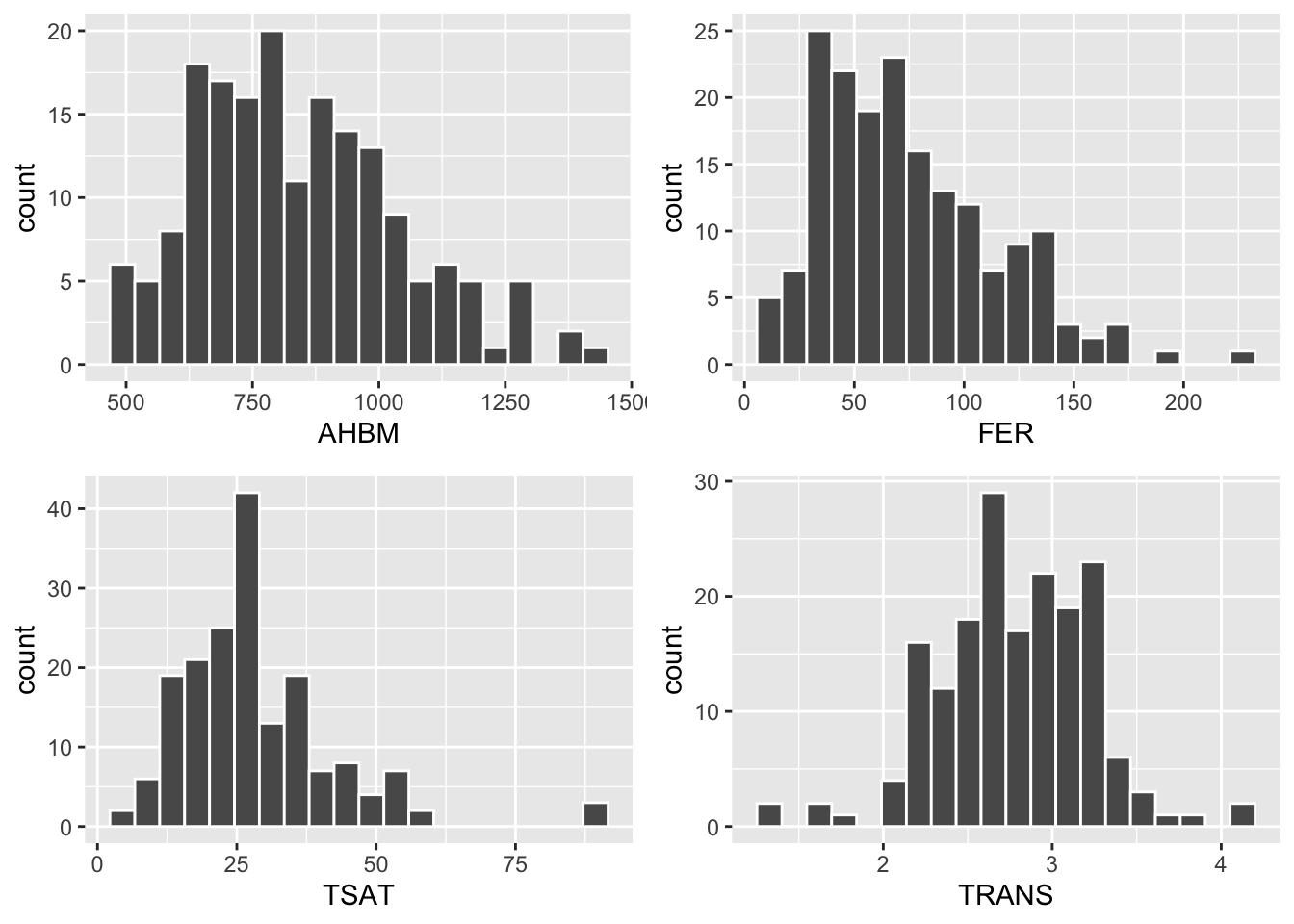
4.3.4 Bivariate summaries
It’s also a good idea to visualise the relationship between any independent variables and the dependent variable (AHBM).
b1 <- ggplot(Hbmass_pre, aes(FER, AHBM)) +
  geom_point() +
  geom_smooth(method = 'lm', se = T)

b2 <- ggplot(Hbmass_pre, aes(TSAT, AHBM)) +
  geom_point() +
  geom_smooth(method = 'lm', se = T)

b3 <- ggplot(Hbmass_pre, aes(FE, AHBM)) +
  geom_point() +
  geom_smooth(method = 'lm', se = T)

b4 <- ggplot(Hbmass_pre, aes(TRANS, AHBM)) +
  geom_point() +
  geom_smooth(method = 'lm', se = T)

b5 <- ggplot(Hbmass_pre, aes(SEX, AHBM)) +
  geom_boxplot() +
  xlab("SEX")

b6 <- ggplot(Hbmass_pre, aes(SUP_DOSE, AHBM)) +
  geom_boxplot() +
xlab("SEX")gridExtra::grid.arrange(b1, b2, b3, b4, b5, b6)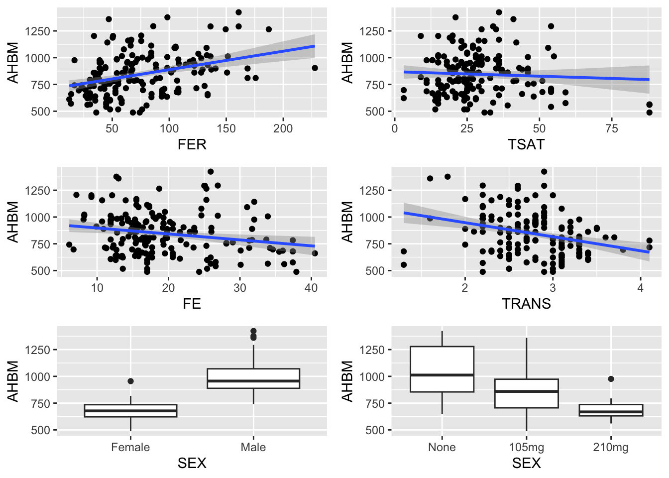
We can include additional factors if we wanted to inspect three-way, four-way, etc., relationships between our variables. For example, numerous studies have identified Sex differences across biological factors. Adding in Sex to our initial visualisations of the data supports this:
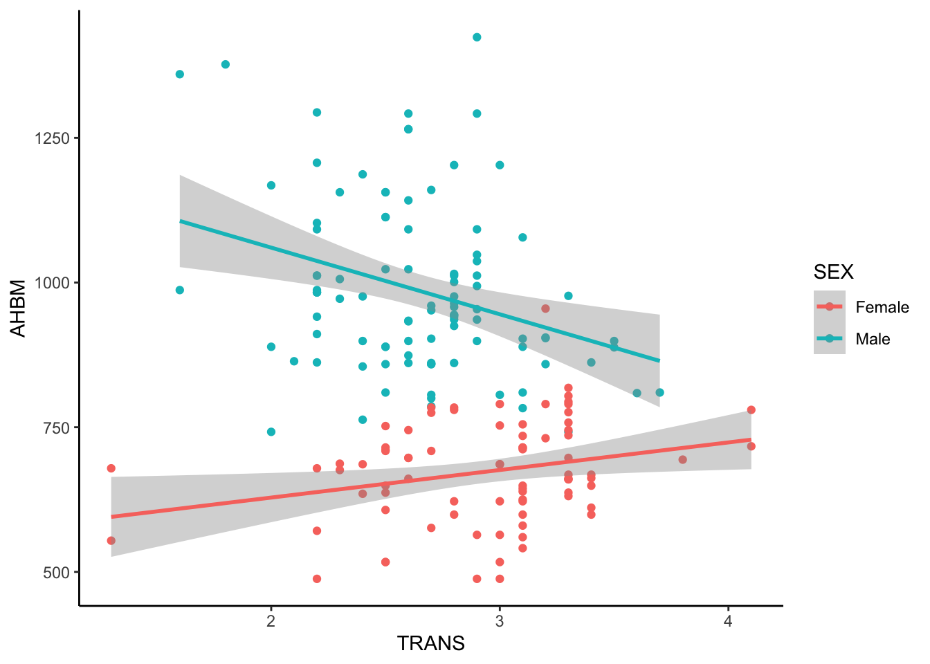
Here, we can see that for females, as TRANS (g/L) increases, AHBM (g) increases as well. On the other hand, we can see the opposite for males - as TRANS increases, AHBM decreases.
4.4 Simple Linear Regression
The term ‘simple linear regression’ refers to linear regression models with only one predictor. Sometimes it may be useful to start with a simple model just to understand the relationship between the outcome and main variable of interest (if there is one) before you start adding more predictors. For example, we will begin by modelling AHBM as a function of FER, that is to say: does one’s ferritin levels (ug/L) influence their absolute Haemoglobin mass (g)? Recall from our bivariate summary that FER appears to have a positive relationship with AHBM. Thus, we would be expecting a positive coefficient estimate for our results.
model1 <- lm(AHBM ~ FER, data = Hbmass_pre)
model1 |> summary()
Call:
lm(formula = AHBM ~ FER, data = Hbmass_pre)

Residuals:
    Min      1Q  Median      3Q     Max
-355.51 -143.09  -23.01  119.86  563.22

Coefficients:
            Estimate Std. Error t value Pr(>|t|)
(Intercept) 715.7441    30.2396  23.669  < 2e-16 ***
FER           1.7242     0.3561   4.843 2.79e-06 ***
---
Signif. codes:  0 '***' 0.001 '**' 0.01 '*' 0.05 '.' 0.1 ' ' 1

Residual standard error: 188.8 on 176 degrees of freedom
Multiple R-squared:  0.1176,    Adjusted R-squared:  0.1126
F-statistic: 23.45 on 1 and 176 DF,  p-value: 2.794e-06
Interpretation
By substituting the values from our output into the equation, we obtain a model for predicting AHBM:
\[AHBM_{i}=715.74+1.72FER_{i}+\epsilon_{i}\]
Our model can thus be interpreted as, absolute Hemoglobin Mass (g) will increase by \(\beta_{1}=1.72g\) for each additional ug/L in one’s Ferritin. The estimated value of the intercept, \(\beta_{0}=715.74\) represents the estimated AHBM value when FER equals 0.
In statistical modeling, the error term serves as a comprehensive representation of various sources of variability that affect the dependent variable but are not explicitly accounted for by the independent variables. This term amalgamates subject-specific, within-subject, technical, and measurement errors into a single entity, denoted as ε (epsilon). While the error term is often treated as a collective measure of unpredictability, it is crucial to recognize that its components can be parsed and estimated separately. In more advanced statistical techniques, such as linear mixed models, the error term can be dissected using random effects. By incorporating random effects into the model, one can capture and quantify the inherent variability arising from individual differences, providing a more nuanced understanding of the data. Future lessons may delve into the intricacies of partitioning and estimating specific components of the error term, shedding light on the nuances of variability within the context of linear mixed models and enhancing the precision of statistical analyses.
Note: the interpretation above is for this sample only, i.e. it would be more correct to say:
For this sample, ABHM was 1.72g greater for each addition ug/L increase in Ferritin.
If we wanted to generalise these results to the overall population, we would have to apply a probabilistic framework for making inferences. For example, the Null Hypothesis Significance Testing (NHST) framework would look at the p-value associated with these estimates (see the output above which shows the p-value for FER to be \(2.79 \times10^{-6}\), or 0.00000279) and compare it to some threshold (commonly set at 0.05) and make a decision on whether of not the results could be deemed statistically significant. Here, the computed p-value (0.00000279) is much smaller than the arbitrarily set threshold of 0.05, so we would have more confidence in generalising these results to the overall population.
In the realm of sport and exercise science, a discernible shift in preference has emerged, favoring interval estimation over null hypothesis significance testing (NHST). Researchers and practitioners in this field increasingly recognize the limitations of NHST in providing a comprehensive understanding of data variability and effect sizes. Interval estimation, on the other hand, offers a more nuanced approach by providing a range of plausible values for an unknown parameter, thereby offering a clearer and more informative perspective on the uncertainty associated with study findings.
Calculating the Confidence Interval
The calculation for the 95% CI in this example is given by:
\[CI_{b_i}=b_i\pm t_{\alpha/2}\times SE_{bi}\]
where:
- \(b_i\) is the estimated coefficient for the predictor variable
- \(t_{\alpha/2}\) is the critical t-value from the t-distribution with \(\alpha/2\) significance level and degrees of freedom (\(df\))
- \(SE_{bi}\) is the standard error of the coefficient
From our output above, the 95% CI would be computed as:
\[1.72 \pm 1.96 \times0.36 = [1.02, 2.43]\] We could have also used the following function to obtain the same results:
confint(model1) 2.5 % 97.5 %
(Intercept) 656.065246 775.422939
FER 1.021552 2.426935With regards to the linear regression, we can say that we expect the true slope of FER on AHBM to fall within the interval 1.02 and 2.43.
Note, we would have even more confidence in this conclusion if the model met certain criteria (commonly referred to as statistical assumptions), which were described in Section 3. To check that these assumptions have been met, we can simply use the check_model() function from the easystats package. Note that the check_model() function provides a range of diagnostic tests. We will only be requesting specific ones for now:
library(easystats)
check_model(
  model1,
  check = c('linearity','homogeneity','normality','outliers')
)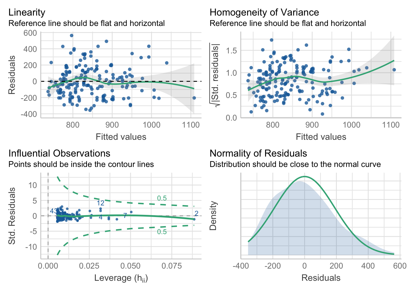
Assumptions interpretation
- The Linearity plot (top-left panel) shows that the residuals are fairly pattern-less, as indicated by the green horizontal line - suggesting that linearity is met.
- The Homogeneity of variance plot (top-right panel) shows shows a slight increase in variability. However, this is only a very minor deviation from 0, so it is unlike to impact the model results too much.
- The Influential Observations plot (bottom-left panel) shows no cases falling outside of cuttoff lines - suggesting that there are no potential influential points of concern.
- The Normality of Residuals (bottom-right panel) shows that residuals are mostly normally distributed - suggesting that normality of residuals is met.
4.5 Multiple Linear Regression
In the previous example we built a linear regression model for AHBM using only FER as a predictor. As the name suggest, multiple linear regression involves building models that contain multiple predictors. As an example, let us now also includeFE (Iron) and TSAT (Transferrin Saturation) into the model. Mathematically, this can be expressed as:
\[Y_{i}=\beta_{0}+\beta_{1}FER+\beta_{2}FE+\beta_{3}TSAT+\epsilon_{i}\]
Similar to before, we need to determine what the values of the \(\beta\) coefficients are, to substitute into the equation.
model2 <- lm(AHBM ~ FER + FE + TSAT, data = Hbmass_pre)
model2 |> summary()
Call:
lm(formula = AHBM ~ FER + FE + TSAT, data = Hbmass_pre)

Residuals:
    Min      1Q  Median      3Q     Max
-367.29 -132.12  -13.85   95.71  497.15

Coefficients:
            Estimate Std. Error t value Pr(>|t|)
(Intercept)  830.417     44.667  18.591  < 2e-16 ***
FER            1.796      0.350   5.131 7.63e-07 ***
FE            -8.106      2.519  -3.218  0.00154 **
TSAT           1.302      1.378   0.945  0.34573
---
Signif. codes:  0 '***' 0.001 '**' 0.01 '*' 0.05 '.' 0.1 ' ' 1

Residual standard error: 183.1 on 174 degrees of freedom
Multiple R-squared:  0.1795,    Adjusted R-squared:  0.1654
F-statistic: 12.69 on 3 and 174 DF,  p-value: 1.536e-07
Based upon the output above we can see that the coefficients are:
- \(\beta_{0}=830.42\)
- \(\beta_{1}=1.80\)
- \(\beta_{2}=-8.11\)
- \(\beta_{3}=1.30\)
Interpretation
Like before, substituting the values from our output into the equation, we obtain a model for predicting AHBM:
\[AHBM_{i}=830.42+1.80FER_{i}-8.11FE_i+1.30TSAT_i+\epsilon_{i}\]
Notice that some \(\beta\) estimates are positive and some are negative. This provides us with an indication the direction of change for the outcome variable.
- absolute Heamoglobin Mass increases by \(\beta_{1}=1.80g\) for each additional ug/L in one’s Ferritin, whilst controlling for FE and TSAT.
- absolute Heamoglobin Mass decreases by \(\beta_{2}=8.11g\) for each additional ug/L in one’s Iron, whilst controlling for FER and TSAT.
- absolute Heamoglobin Mass increases by \(\beta_{3}=1.30g\) for each additional % in one’s Transferrin Saturation, whilst controlling for FER and FE.
Similar to the simple linear regression example, we can inspect the associated p-values and 95% confidence intervals for each predictor from the output above. If these values are less than the chosen threshold (e.g. 0.05) then we have confidence in inferring these results to the larger population. In this example, FER and FE have p-values less than 0.05, so we can say that these results are statistically significant. Looking at the confidence intervals:
confint(model2) 2.5 % 97.5 %
(Intercept) 742.257999 918.576775
FER 1.105154 2.486704
FE -13.078068 -3.134101
TSAT -1.416441 4.021285From the output above, we can say that:
- The true slope for
FERonAHBM, whilst controlling forFEandTSATis estimated to fall within the interval 1.11 to 2.49. This interval is positive, so we would infer a 1.11 to 2.49 increase inAHBMfor each additional increase inFER. - The true slope for
FEonAHBM, whilst controlling forFERandTSATis estimated to fall within the interval -13.08 to -3.13. This interval is negative, so we would infer a 13.08 to 3.13 decrease inAHBMfor each additional increase inFE. - The true slope for
TSATonAHBMis uncertain, as it ranges from -1.42 (a decrease) to 4.02 (an increase). This aligns with the non-significant p-value observed for this predictor.
Similar to previous example, we should also check the statistical assumptions to ensure that our model is valid. Multiple linear regression requires two additional assumptions to be met for a model to be valid:
Assumption 5: Multivariate normality
Multivariate normality assumes data from multiple variables follow a multivariate normal distribution. In statistics, a normal distribution (or Gaussian distribution) is a symmetric, bell-shaped probability distribution that is characterized by its mean and standard deviation. The multivariate normal distribution extends this concept to multiple dimensions, where there is a vector of means and a covariance matrix that describes the relationships between the variables.
There are many different methods for checking this assumption. The MVN package contains different methods for assessing multivariate normality. In the code below, we illustrate how to use this package with the Henze-Zirkler’s test.
library(MVN)

# Subset the data to only include variables in the model
data_check <-
  Hbmass_pre |>
  select(AHBM, FER, FE, TSAT)

# Run the MVN test
res <- mvn(data_check, mvnTest = 'hz')

# Show the results
res$multivariateNormality
Test HZ p value MVN
1 Henze-Zirkler 3.135144 0 NOOne of the most common reasons for multivariate normality being violated is the presence of multivariate outliers. The MVN package checks for these by calculating robust Mahalanobis distances (which is simply a metric that calculates how far away each observation is to the center of the multivariate space).
mvn(data_check, mvnTest = 'hz',
    multivariateOutlierMethod = 'adj')
In the output above, we can observe 30 cases as multivariate outliers. A potential next step would be to inspect these observations and determine if they should be removed or retained in the data set. To keep this example simple, we will choose to retain these observations for now.
Assumption 6: Multicollinearity
Multicollinearity assumes that the predictor variables are not perfectly correlated with each other, as perfect multicollinearity can lead to instability and unreliable estimates in the regression model. Multicollinearity can manifest when two or more independent variables are highly correlated, making it challenging to isolate the individual effects of each predictor on the dependent variable. This can result in inflated standard errors, making it difficult to discern the true significance of the variables.
One essential diagnostic tool to assess multicollinearity is the Variance Inflation Factor (VIF). VIF quantifies the extent to which the variance of an estimated regression coefficient is increased due to multicollinearity. It is calculated for each predictor variable, and a high VIF value indicates a problematic level of multicollinearity. In simpler terms, a high VIF suggests that the variable may be too closely related to other predictors, making it challenging to discern its unique contribution to the model.
Conversely, tolerance is another metric used to evaluate multicollinearity. Tolerance is the reciprocal of VIF and ranges between 0 and 1. A low tolerance value indicates high multicollinearity, implying that a significant proportion of the variance in a predictor can be explained by other predictors in the model. In the presence of multicollinearity, tolerance values tend to be close to zero, highlighting the challenges in isolating the independent contribution of each predictor.
We can use the check_collinearity() function from the performance package to compute the VIF and Tolerence for us:
library(performance)
check_collinearity(model2)
# Check for Multicollinearity
Low Correlation
Term VIF VIF 95% CI Increased SE Tolerance Tolerance 95% CI
FER 1.03 [1.00, 7.44] 1.01 0.97 [0.13, 1.00]
FE 1.86 [1.55, 2.34] 1.36 0.54 [0.43, 0.65]
TSAT 1.89 [1.57, 2.38] 1.37 0.53 [0.42, 0.64]We can also use the ggpairs() function from the GGally package to visualise the relationship among all of the predictors:
library(GGally)
ggpairs(Hbmass_pre,
        columns = c('FER','FE','TSAT'))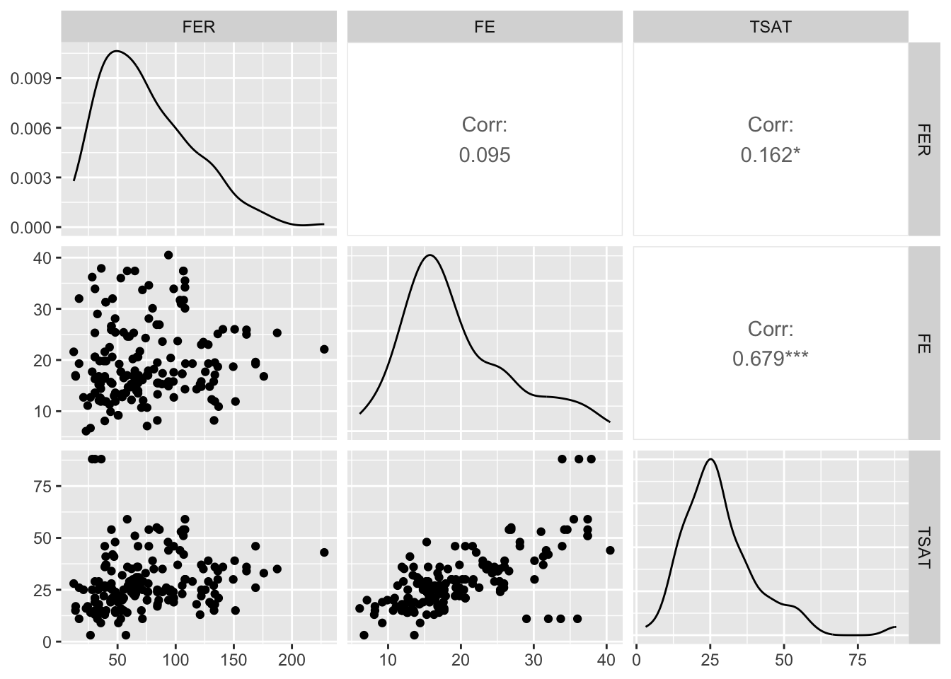
4.6 Multiple Linear Regression with interactions
In multiple regression, interaction terms play a pivotal role in capturing the combined or interactive effect of two or more predictor variables on the dependent variable. Interaction terms are introduced by multiplying the values of two or more predictors, creating new variables that represent the joint impact of the original predictors. These terms enable researchers to investigate whether:
the relationship between a predictor and the dependent variable varies depending on the level of another predictor.
The inclusion of interaction terms helps to uncover nuanced and context-dependent patterns in the data that may be overlooked when considering individual predictors in isolation. Identifying and interpreting interaction effects is crucial for a comprehensive understanding of complex relationships within a multiple regression framework, allowing researchers to account for potential synergies or moderating influences that can significantly influence the overall model.
Interaction terms in multiple regression can take various forms depending on the types of variables involved. several common types are provided below. When investigating interactions, it is advised to visualise the relationship first, before looking at the model results.
4.6.1 Categorical-Categorical Interaction:
Interaction between two categorical variables explores whether the relationship between them is different across different categories. Using the current data, we could explore how SEX interacts with SUP_DOSE to influence AHBM. To begin, let us inspect this relationship visually:
ggplot(Hbmass_pre, aes(SUP_DOSE, AHBM, fill = SEX)) +
  geom_boxplot() +
  geom_jitter() +
  facet_wrap(~SEX) +
  theme(legend.position = 'none')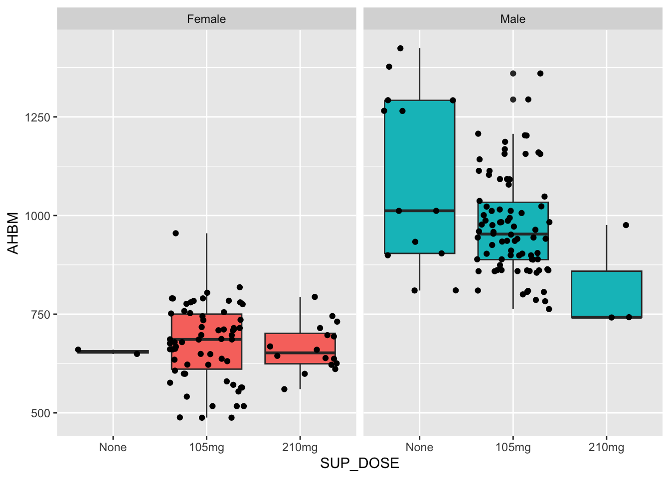
One question we might ask is “Is there a relationship between SUP_DOSE and AHBM?” Looking at the plot we might say that it depends on SEX. For females, AHBM appears to be consistent across the three SUP_DOSE groups. On the other hand, for males, AHBM appears to be decreasing as SUP_DOSE increases (note: caution is advised when interpreting this because there are very few observations for females and none; and males and 210mg, n = 2 and n = 3 respectively).
To include an interaction term in our models, we would multiply them together. For example:
model3 <- lm(AHBM ~ SEX + SUP_DOSE + SEX*SUP_DOSE, data = Hbmass_pre)
model3 |> summary()
Call:
lm(formula = AHBM ~ SEX + SUP_DOSE + SEX * SUP_DOSE, data = Hbmass_pre)

Residuals:
    Min      1Q  Median      3Q     Max
-289.62  -84.72   -6.56   73.06  386.28

Coefficients:
                      Estimate Std. Error t value Pr(>|t|)
(Intercept)             654.50      85.88   7.621 1.62e-12 ***
SEXMale                 445.12      92.25   4.825 3.07e-06 ***
SUP_DOSE105mg            21.11      87.25   0.242   0.8091
SUP_DOSE210mg            10.56      91.09   0.116   0.9078
SEXMale:SUP_DOSE105mg  -147.01      94.49  -1.556   0.1216
SEXMale:SUP_DOSE210mg  -290.18     119.79  -2.422   0.0165 *
---
Signif. codes:  0 '***' 0.001 '**' 0.01 '*' 0.05 '.' 0.1 ' ' 1

Residual standard error: 121.5 on 172 degrees of freedom
Multiple R-squared:  0.6432,    Adjusted R-squared:  0.6328
F-statistic: 62 on 5 and 172 DF, p-value: < 2.2e-16confint(model3) 2.5 % 97.5 %
(Intercept) 484.9881 824.01192
SEXMale 263.0304 627.20039
SUP_DOSE105mg -151.1114 193.33718
SUP_DOSE210mg -169.2320 190.35704
SEXMale:SUP_DOSE105mg -333.5100 39.49243
SEXMale:SUP_DOSE210mg -526.6159 -53.73988Using the output from the interaction model, the regression equation for this model would be:
\[AHBM=654.50+445.12(SEX)+21.11(SDOSE_{105})+10.56(SDOSE_{210})-\\147.01(SEX*SDOSE_{105})-290(SEX*SDOSE_{210})\]
Recall that our codes for these variables are:
SEX: 0 = Female, 1 = MaleSUP_DOSE: 0 = None, 1 = 105mg, 2 = 210mg
Thus if we want to estimate the effect for Females and None, we would substitute 0 into the equation wherever we see SEX, and remove these SUP_DOSE effects (because they correspond to 105mg and 210mg). This leaves us with:
\[AHBM=654.50+445.12(0)+0-0-0=654.50\]
Notice here, that this is the Intercept value from our regression model. When we only have categorical variables in our model, the intercept is equivalent to when all factors are equal to 0. You can also have a look at the box plot we generated earlier for this relationship - the mean value for Females and None should be 654.50.
Now, suppose we wanted to estimate AHBM for males on a supplement dose of 210mg. Are formula would become:
\[AHBM=654.50+445.12(1)+0+10.56-290(1)=809.62\]
Again, have a look at the plot we generated. If you draw a y-intercept at 809, this should represent the mean for Males on the 210mg dose. We can repeat the process to determine the estimated AHBM value for different combinations of the categorical predictors.
4.6.2 Categorical-Continuous Interaction:
This type involves the interaction between a categorical variable and a continuous variable. Typically it is to explore if the slope in the continuous variable differs for the levels within the categorical variable. In the context of this study, suppose we wanted to look at the interaction between SEX and TRANS. Like before, let’s start with visualising this relationship:
ggplot(Hbmass_pre, aes(TRANS, AHBM, color = SEX)) +
  geom_point() +
  geom_smooth(method = 'lm', se=T) +
  facet_wrap(~SEX)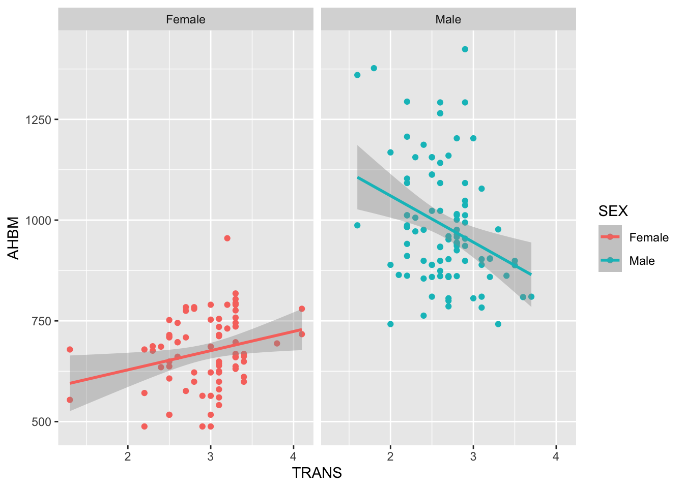
We might have a question is there a relationship between TRANS and AHBM?
Looking at the plot, we can say it depends on SEX. For females, as TRANS increases, AHBM increases. For males, as TRANS increases, AHBM decreases.
Running a linear regression for this model will produce the following output:
model4 <- lm(AHBM ~ SEX + TRANS + SEX*TRANS, data = Hbmass_pre)
model4 |> summary()
Call:
lm(formula = AHBM ~ SEX + TRANS + SEX * TRANS, data = Hbmass_pre)

Residuals:
    Min      1Q  Median      3Q     Max
-318.36  -67.41  -20.00   64.95  467.32

Coefficients:
              Estimate Std. Error t value Pr(>|t|)
(Intercept)     533.08      84.90   6.279 2.64e-09 ***
SEXMale         757.69     117.37   6.456 1.04e-09 ***
TRANS            47.67      28.56   1.669  0.09689 .
SEXMale:TRANS  -162.87      41.60  -3.915  0.00013 ***
---
Signif. codes:  0 '***' 0.001 '**' 0.01 '*' 0.05 '.' 0.1 ' ' 1

Residual standard error: 121 on 174 degrees of freedom
Multiple R-squared:  0.6415,    Adjusted R-squared:  0.6353
F-statistic: 103.8 on 3 and 174 DF, p-value: < 2.2e-16confint(model4) 2.5 % 97.5 %
(Intercept) 365.508837 700.64393
SEXMale 526.040993 989.33393
TRANS -8.697422 104.02868
SEXMale:TRANS -244.977788 -80.75699The model thus becomes:
\[AHBM=533.08+757.69(SEX)+47.67(TRANS)-162.87(SEX*TRANS)\]
Using this output, we can derive separate equations for females and males:
\[AHBM_{females}=533.08+0+47.67(TRANS)-167.87(0) \\ = 533.08 +47.67(TRANS)\]
\[AHBM_{males}=533.08+757.69(1)+47.67(TRANS)-162,87(TRANS) \\ = 1290.77-115.2(TRANS)\]
From these equations we can see that the intercept for females and males is 533.08 and 1290.77 respectively. The slope in these equations tell us that for females, ever additional increase in TRANS, equates to a 47.67 increase in AHBM. Conversely for males, every additional increase in TRANS leads to a 115.2 decrease in AHBM. This matches with the plot we generated earlier.
4.6.3 Continuous-Continuous Interaction:
Interaction between two continuous variables explores whether their combined effect on the dependent variable is different at different levels. Exploring and interpreting continuous-continuous interactions often involves investigating the relationship between two continuous variables at different levels, such as varying values around the mean, one standard deviation above and below the mean, or other meaningful intervals. This process allows for a more nuanced understanding of how the interaction effect changes across the range of the variables. This can easily be done with the interact_plot() function from the interactions package.
As an example, let’s look at how the relationship between FE and AHBM might depend on TSAT.
library(interactions)
model5 <- lm(AHBM ~ FE + FER + FE*TSAT, data = Hbmass_pre)
interact_plot(model5, pred = FE, modx = TSAT)+theme(legend.position = 'bottom')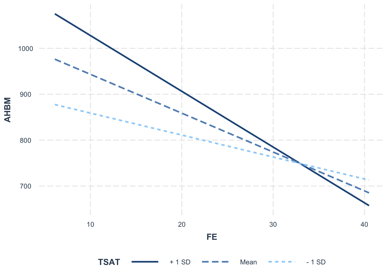
From these plots, we can see that the interaction effect is showing a negative slope. This represents the change in the effect of the predictor (FE) on the outcome (AHBM) for a one-unit increase in the moderator (TSAT). The plot also shows 1 standard deviation above and below the centered-mean for the moderator. This is useful for explaining how high and low values of the moderator can influence the relationship between FE and AHBM. For example: for athletes with lower TSAT values (represented by the - 1 SD line), the relationship between FE and AHBM decreases at a lower rate compared to athletes with a higher TSAT value (represented by the + 1 SD line). We can also see that the - 1 SD and + 1 SD lines cross at approximately FE = 32, suggesting that the relationship between FE and AHBM varies at different levels of TSAT.
Looking at the output for our model, we can see that this interaction effect is statistically significant:
model5 |> summary()
Call:
lm(formula = AHBM ~ FE + FER + FE * TSAT, data = Hbmass_pre)

Residuals:
    Min      1Q  Median      3Q     Max
-395.00 -114.78  -18.31   86.23  463.57

Coefficients:
            Estimate Std. Error t value Pr(>|t|)
(Intercept) 654.6145    86.3004   7.585 1.95e-12 ***
FE           -0.7878     3.9649  -0.199   0.8427
FER           1.6050     0.3547   4.525 1.12e-05 ***
TSAT          8.8297     3.4553   2.555   0.0115 *
FE:TSAT      -0.2680     0.1131  -2.370   0.0189 *
---
Signif. codes:  0 '***' 0.001 '**' 0.01 '*' 0.05 '.' 0.1 ' ' 1

Residual standard error: 180.7 on 173 degrees of freedom
Multiple R-squared:  0.2053,    Adjusted R-squared:  0.1869
F-statistic: 11.17 on 4 and 173 DF,  p-value: 4.371e-08
4.6.4 Confidence Intervals vs. Prediction Intervals
In linear regression analysis, both confidence intervals (CIs) and prediction intervals (PIs) are important statistical tools that provide valuable insights into the model’s predictions. While they might seem similar at first glance, there are key differences between them that are essential for accurate interpretation. Understanding these differences is crucial for drawing meaningful conclusions from the data and making appropriate predictions.
Confidence Intervals
A confidence interval represents the range within which we expect the average value of the dependent variable to fall, given specific values of the predictor variables, with a certain level of confidence (e.g. 95%). It focuses on estimating the mean response for a particular set of predictors. In other words, it tells us about the precision of our regression model in predicting the expected value of the outcome variable.
Using our model5 as an example, the 95% confidence interval for FER would be 95% CI = [0.905 to 2.305]
confint(model5) 2.5 % 97.5 %
(Intercept) 484.2772497 824.95170146
FE -8.6134935 7.03794710
FER 0.9048488 2.30510063
TSAT 2.0097091 15.64963246
FE:TSAT -0.4912451 -0.04477254This interval suggests that, with 95% confidence, the true effect of FER on AHBM lies between 0.9048 and 2.3051, holding all other variables in the model constant.
Prediction Intervals
A prediction interval, on the other hand, estimates the range within which a single new observation of the dependent variable is likely to fall, given specific values of the predictor variables. Prediction intervals are generally wider than confidence intervals because they account not only for the uncertainty in estimating the mean but also for the variability of individual observations around that mean.
For example, suppose we have a new participant with specific characteristics: for instance, FER = 1.5, FE = 2, and TSAT = 10.
new_data <- data.frame(FE = 2, FER = 1.5, TSAT = 10)Using these values, we can apply our regression model to predict the dependent variable for this individual:
predict(model5, newdata = new_data, interval = "prediction", level = 0.95) fit lwr upr
1 738.3829 364.4675 1112.298This output tells us that the predicted response for the new participant is approximately 738.38, with a 95% prediction interval ranging from 364.47 to 1112.30. This range accounts for both the uncertainty in the mean prediction and the variability in individual observations.
Practical Implications
In practice, you should use confidence intervals when you want to understand the average impact of predictors in your model (e.g the average effect of FER on AHBM). Use prediction intervals when you want to estimate the range of possible outcomes for individual predictions (e.g., predicting the AHBM of a specific person given their FE, FER and TSAT values).
4.7 Building models
As you may have noted in the previous exercises, we deliberately avoided fitting models with all available variables simultaneously. The reason behind this strategic approach lies in mitigating the risk of overfitting. Overfitting occurs when a model learns not only the underlying patterns in the training data but also captures random noise, making it overly complex and tailored specifically to the training set. While such a model may perform exceptionally well on the training data, it often fails to generalize to new, unseen data, leading to unreliable predictions. By selectively choosing variables and employing techniques such as stepwise regression or regularization methods (more on these in later lessons), we aim to strike a balance between model complexity and predictive accuracy.
Selection of the appropriate model involves a nuanced understanding of the problem domain, the nature of the data, and the goals of the analysis. An expert in the field plays a crucial role in this process, leveraging domain knowledge and experience to make informed decisions. While a computerized approach facilitates model selection through algorithmic exploration, the nuanced interpretation of results and contextual understanding require human expertise. Experts guide the selection process by considering factors such as model assumptions, interpretability, computational efficiency, and the robustness of predictions.
4.7.1 Model parsimony
Model parsimony is the principle of favoring simpler models that achieve a balance between explanatory power and simplicity. A parsimonious model uses the fewest variables or parameters necessary to adequately describe the observed data without overfitting. One way to formalize this principle in model selection is through the Bayesian Information Criterion (BIC). The Bayesian Information Criterion is a metric that balances goodness of fit with model complexity. In the context of multiple regression, BIC penalizes models for having more parameters. The BIC formula is given by:
In the context of model parsimony, a lower BIC indicates a more parsimonious model that achieves a good fit with fewer parameters. When comparing models, one should prefer the model with the lowest BIC, as it strikes a balance between capturing the complexity in the data and avoiding unnecessary elaboration.
4.7.2 Model Fit
When building our models, one consideration to make is the model fit. Model fit examines how well the chosen model explains the variation in the dependent variable based on the included independent variable(s). In this example, how well does the model explain AHBM. There are different metrics that we can use to assess model fit, with a few popular choices being:
R-squared: R-squared is a common metric that quantifies the proportion of the variance in the dependent variable explained by the independent variables. A higher R-squared suggests a better fit, but it should be interpreted in conjunction with other diagnostics.
Adjusted R-squared: Adjusted R-squared adjusts for the number of predictors in the model, penalizing the inclusion of unnecessary variables. It provides a more reliable measure, especially in models with multiple predictors.
Comparing a few metrics across all models that we have built so far in this lesson, allows us to compare and ultimately choose a final model.
| Model | Effects | R.squared | Adj.R.squared | BIC |
|---|---|---|---|---|
| 1 | FER | 0.1175768 | 0.1125631 | 2384.370 |
| 2 | FER + FE + TSAT | 0.1795098 | 0.1653634 | 2381.780 |
| 3 | SEX + SUP_DOSE + SEX*SUP_DOSE | 0.6431640 | 0.6327909 | 2243.937 |
| 4 | SEX + TRANS + SEX*TRANS | 0.6415130 | 0.6353322 | 2234.395 |
| 5 | FE + FER + FE*TSAT | 0.2053037 | 0.1869292 | 2381.277 |
Notice that both R2 and adjusted R2 values are largest in models 3 and 4, both of which include the predictor SEX. Additionally, the BIC is relatively lower in these two models compared to the others. While there might be a temptation to choose one of these models based on statistical metrics, it’s crucial to emphasize that the final model selection should always be supported by theory and made in consultation with a domain-specific expert. This is because some models that may appear statistically favorable may lack biological justification, or they may include variables that should not be combined in a single model
4.7.3 Splitting the data
The models constructed so far have used the complete dataset for both training and evaluation, posing a potential risk of overfitting, where the model may perform well on the training data but struggle with new, unseen data. To address this issue, one recommended approach is to split the data into training and testing sets. By doing so, we can assess various metrics, such as R squared mentioned earlier, on both sets. The objective is to ensure that fit metrics remain relatively consistent across both sets. For instance, if the R squared is significantly larger in the training set compared to the testing set, it may indicate a problem with overfitting.
To demonstrate this, we will explore a tidymodels workflow on our third model, which included main effects for SEX and SUP_DOSE, and an interaction effect between these two variables.
library(tidymodels)

# Step 1. Split the data
set.seed(1)
splits <- initial_split(Hbmass_pre)
Hbmass_pre_training <- training(splits)
Hbmass_pre_testing <- testing(splits)
# Step 2. Fit the model
lm_fit <-
linear_reg() |>
fit(AHBM ~ SEX + SUP_DOSE + SEX*SUP_DOSE, data = Hbmass_pre_training)# Step 3. Compare metrics (here R^2) for both training and testing sets
bind_rows(
# Find R^2 value for training
lm_fit |>
predict(Hbmass_pre_training) |>
mutate(Truth = Hbmass_pre_training$AHBM) |>
rsq(Truth, .pred),
# Find R^2 value for testing
lm_fit |>
predict(Hbmass_pre_testing) |>
mutate(Truth = Hbmass_pre_testing$AHBM) |>
rsq(Truth, .pred)
) |>
mutate(model = c("Train", "Test"))# A tibble: 2 × 4
.metric .estimator .estimate model
<chr> <chr> <dbl> <chr>
1 rsq standard 0.659 Train
2 rsq standard 0.555 Test Notice in this example that the R2 for the training set (R2 = .659) is much larger than the R2 value for the testing set (R2 = .555). There can be a number of different reasons for this. For example, the model may have learned specific patterns or noise in the training data that do not generalize well to new, unseen data. This phenomenon is known as overfitting, where the model becomes too tailored to the training set and struggles to perform effectively on diverse data. Another possible reason could be the presence of outliers or anomalies in the testing set that were not adequately represented in the training data. Additionally, the model’s complexity may be a contributing factor; an overly complex model might fit the training data too closely, leading to poor generalization. Finally, it might just be due to random luck, as the process for creating the training and testing sets is based upon randomly sampling from the full data set.
4.7.4 Cross validation
To address the challenges highlighted by the disparity in R2 values between the training and testing sets, cross-validation emerges as a valuable tool. Cross-validation involves systematically partitioning the dataset into multiple subsets, training the model on different combinations of these subsets, and evaluating its performance across various folds. By doing so, cross-validation provides a more comprehensive assessment of the model’s ability to generalize. In the context of our example, cross-validation would entail repeatedly splitting the data into training and validation sets, allowing the model to learn from different portions of the data. This process helps to smooth out the impact of specific data configurations and minimizes the influence of outliers or random variations in the initial train-test split. The average performance over multiple folds gives a more reliable estimate of how well the model is expected to perform on new, unseen data, offering a robust solution to the challenges associated with overfitting, outlier sensitivity, and random chance in the data partitioning process.
An example of kfolds cross validation is demonstrated below using the tidymodels framework:
# Split data (we did this before, but we'll do this again for practice)
data_splits <- initial_split(Hbmass_pre)
Hbmass_pre_training <- training(data_splits)
Hbmass_pre_testing <- testing(data_splits)
# Create a cross-validation set on the training data
cv_folds <- vfold_cv(Hbmass_pre_training)# Define a model specification
lm_spec <- linear_reg()# Fit the model
lm_fit <- lm_spec |>
fit(AHBM ~ SEX + SUP_DOSE + SEX*SUP_DOSE, data = Hbmass_pre_training)# Perform cross validation
cv_results <-
fit_resamples(
lm_spec,
AHBM ~ SEX + SUP_DOSE + SEX*SUP_DOSE,
cv_folds,
metrics = metric_set(rsq),
control = control_resamples(save_pred = T)
)The code above creates 10 folds (which is the default number of folds, but we can change this if needed) and stores the results in a list:
cv_results# Resampling results
# 10-fold cross-validation
# A tibble: 10 × 5
splits id .metrics .notes .predictions
<list> <chr> <list> <list> <list>
1 <split [119/14]> Fold01 <tibble [1 × 4]> <tibble [0 × 3]> <tibble [14 × 4]>
2 <split [119/14]> Fold02 <tibble [1 × 4]> <tibble [1 × 3]> <tibble [14 × 4]>
3 <split [119/14]> Fold03 <tibble [1 × 4]> <tibble [1 × 3]> <tibble [14 × 4]>
4 <split [120/13]> Fold04 <tibble [1 × 4]> <tibble [0 × 3]> <tibble [13 × 4]>
5 <split [120/13]> Fold05 <tibble [1 × 4]> <tibble [0 × 3]> <tibble [13 × 4]>
6 <split [120/13]> Fold06 <tibble [1 × 4]> <tibble [0 × 3]> <tibble [13 × 4]>
7 <split [120/13]> Fold07 <tibble [1 × 4]> <tibble [0 × 3]> <tibble [13 × 4]>
8 <split [120/13]> Fold08 <tibble [1 × 4]> <tibble [0 × 3]> <tibble [13 × 4]>
9 <split [120/13]> Fold09 <tibble [1 × 4]> <tibble [0 × 3]> <tibble [13 × 4]>
10 <split [120/13]> Fold10 <tibble [1 × 4]> <tibble [0 × 3]> <tibble [13 × 4]>
There were issues with some computations:
- Warning(s) x2: prediction from rank-deficient fit; consider predict(., rankdefic...
Run `show_notes(.Last.tune.result)` for more information.We can extract out these results with:
cv_results |> unnest(.metrics)# A tibble: 10 × 8
splits id .metric .estimator .estimate .config .notes
<list> <chr> <chr> <chr> <dbl> <chr> <list>
1 <split [119/14]> Fold01 rsq standard 0.747 Preprocessor1_… <tibble>
2 <split [119/14]> Fold02 rsq standard 0.201 Preprocessor1_… <tibble>
3 <split [119/14]> Fold03 rsq standard 0.367 Preprocessor1_… <tibble>
4 <split [120/13]> Fold04 rsq standard 0.539 Preprocessor1_… <tibble>
5 <split [120/13]> Fold05 rsq standard 0.577 Preprocessor1_… <tibble>
6 <split [120/13]> Fold06 rsq standard 0.737 Preprocessor1_… <tibble>
7 <split [120/13]> Fold07 rsq standard 0.610 Preprocessor1_… <tibble>
8 <split [120/13]> Fold08 rsq standard 0.785 Preprocessor1_… <tibble>
9 <split [120/13]> Fold09 rsq standard 0.753 Preprocessor1_… <tibble>
10 <split [120/13]> Fold10 rsq standard 0.767 Preprocessor1_… <tibble>
# ℹ 1 more variable: .predictions <list>In the above, we can see the different R2 values for the 10 folds of our cross validated set. To inspect the average R2 value we can use:
cv_results |> collect_metrics()# A tibble: 1 × 6
.metric .estimator mean n std_err .config
<chr> <chr> <dbl> <int> <dbl> <chr>
1 rsq standard 0.608 10 0.0618 Preprocessor1_Model15 Conclusion and Reflection
In conclusion, delving into linear regression provides a robust framework for understanding and analyzing relationships within sport science data. By scrutinizing the assumptions and interpreting the coefficients, we’ve gained valuable insights into the dynamics between variables, paving the way for informed decision-making in athletic performance and training optimization. The ability to assess linearity, independence, normality, and equality of variances equips us with th e tools to ensure the reliability of our models. As we decipher the implications of regression coefficients, we unlock a deeper comprehension of how factors such as training intensity, player performance, and injury rates interconnect. Armed with this knowledge, sport scientists and coaches are better positioned to tailor training programs, enhance player development strategies, and contribute to the overall advancement of athletic performance and well-being.
With that said, whilst linear regression is an invaluable tool for exploring relationships within sport science data, it represents just the tip of the iceberg in the realm of regression modeling. The versatility of regression extends beyond the linear framework, offering a diverse array of models to address various types of data and outcomes. Logistic regression, for instance, is well-suited for binary outcomes, making it applicable in scenarios such as predicting injury occurrence. Polynomial regression accommodates non-linear relationships, allowing for a more nuanced exploration of complex patterns in sports data. The exploration of other regression models, such as ridge regression or lasso regression, brings forth techniques for handling multicollinearity and feature selection. As we venture deeper into these advanced regression methods, we unlock new possibilities for understanding and predicting outcomes in sport science, showcasing the rich landscape of statistical tools available to researchers and practitioners alike.
6 Knowledge Spot Check
What type of outcome variable is typically used in linear regression?
- Continuous
- Binary
- Count
- Ordinal
- Continuous
Linear regression is commonly used when the outcome variable is continuous, such as weight, height, or temperature. It models the relationship between one or more predictor variables and the continuous outcome variable.
In a multiple regression analysis, if the coefficient for a predictor variable is 3.5, what does this imply about the relationship between that predictor and the outcome variable, assuming all other variables are held constant?
- For every one-unit increase in the predictor variable, the outcome variable is expected to increase by 3.5 units, assuming all other variables are held constant.
- For every one-unit increase in the predictor variable, the outcome variable is expected to increase by 3.5 units, regardless of the values of other predictor variables.
- The outcome variable will decrease by 3.5 units for every one-unit increase in the predictor variable.
- The coefficient of 3.5 indicates a weak relationship between the predictor variable and the outcome variable.
- For every one-unit increase in the predictor variable, the outcome variable is expected to increase by 3.5 units, assuming all other variables are held constant.
In multiple regression, the coefficient for a predictor variable represents the expected change in the outcome variable for a one-unit increase in that predictor, while controlling for the effects of all other predictor variables in the model.
What does the assumption of normality refer to in the context of regression analysis?
- The dependent variable must be normally distributed.
- The residuals of the regression model should be normally distributed.
- The predictor variables must be normally distributed.
- All of the variables must be normally distributed.
- The residuals of the regression model should be normally distributed.
The assumption of normality in regression analysis specifically pertains to the distribution of the residuals (the differences between observed and predicted values). A common misconception is that this assumption relates to the dependent variable being normally distributed.
What does heteroscedasticity indicate in the context of linear regression?
- The variability of the outcome variable is constant across all levels of the predictor variables.
- The variability of the outcome variable is greater at certain levels of the predictor variables.
- The outcome variable follows a normal distribution rather than a uniform distribution.
- The outcome variable is perfectly predicted by the predictor variables.
- The variability of the outcome variable is greater at certain levels of the predictor variables.
Heteroscedasticity in linear regression occurs when the variability of the outcome variable is not constant across all levels of the predictor variables, leading to inefficient estimates and potentially misleading hypothesis tests if not addressed.
In linear regression, how do confidence intervals and prediction intervals differ in their interpretation?
- Confidence intervals provide a range of values for the population parameter, while prediction intervals provide a range of values for a single future observation.
- Confidence intervals apply to individual data points, while prediction intervals apply to the mean response of the outcome variable.
- Confidence intervals are wider than prediction intervals because they account for variability in the outcome variable.
- Confidence intervals are used for categorical outcomes, while prediction intervals are used for continuous outcomes.
- Confidence intervals provide a range of values for the population parameter, while prediction intervals provide a range of values for a single future observation.
In linear regression, confidence intervals estimate the range within which we expect the true population parameter (e.g., the mean response) to fall, while prediction intervals estimate the range within which we expect a single new observation to fall. Prediction intervals are generally wider than confidence intervals due to the additional variability associated with predicting individual outcomes.