Regression Modeling Strategies 2 - Poisson Regression
Modeling Count Data in Sports Science
Abstract
Poisson regression stands as a crucial statistical methodology frequently employed in sports science for the analysis of count data and the exploration of relationships between variables. In the realm of sports, this modeling technique proves invaluable for delving into scenarios where the outcome of interest is a count variable, such as the number of goals scored, injuries sustained, or penalties incurred during a game. Unlike linear regression, Poisson regression is specifically tailored for situations where the dependent variable represents counts of events within fixed time intervals or areas. By modeling the distribution of these discrete events, sports researchers can gain insights into the factors influencing the frequency of occurrences. For example, in soccer analytics, Poisson regression might be applied to understand how various team strategies, player characteristics, or environmental conditions contribute to the number of goals scored in a match. This approach allows sports scientists to draw meaningful conclusions from count data, providing a statistical framework to optimize tactics, minimize risks, and enhance overall performance and safety in athletic contexts.
Keywords
Poisson regression, count data, overdispersion, negative binomial regression, zero-inflated models, event modeling, R, generalized linear models (GLM), sports statistics, count outcomes, log-linear modeling, t_symp_score, incident rate ratio (IRR), dispersion parameter.
Lesson’s Level
The level of this lesson is categorized as BRONZE.
Lesson’s Main Idea
- Understanding when to use Poisson regression models and their extensions for analyzing count data in sports science.
- Exploring the concepts of equidispersion and overdispersion and learning how to address them using quasi-Poisson and negative binomial regression.
- Examining zero-inflated models and their applications for data with excess zeros.
Dataset Used In This Lesson
In this lesson, we use the HansIll dataset from the speedsR package, an R data package specifically designed for the SPEEDS project. This package provides a collection of sports-specific datasets, streamlining access for analysis and research in the sports science context.
1 Learning Outcomes
By the end of this lesson, you will have developed the ability to:
Model Count Data: Understand the key concepts of Poisson regression, including its assumptions and extensions to handle overdispersion and excess zeros.
Construct and Extend Models: Build Poisson regression models in R and extend them using quasi-Poisson, negative binomial, and zero-inflated models.
Interpret Model Outputs: Interpret coefficients, incidence rate ratios (IRRs), and confidence intervals, and assess their significance in the context of sports science.
Evaluate Model Fit: Apply diagnostic tools to check assumptions and evaluate the goodness-of-fit of count models.
Analyze Count Data in Context: Explore real-world sports applications, such as predicting days sick or analyzing player performance metrics, while addressing overdispersion and zero-inflation challenges.
2 Introduction: Poisson Regression
Poisson regression is a versatile and widely utilized statistical technique designed for modeling relationships between variables, particularly when the dependent variable represents counts of events within fixed intervals or areas. This methodology is particularly well-suited for scenarios where the outcome of interest is a non-negative integer, such as the number of goals scored in a soccer match, incidents of player injuries, or the count of penalties during a game.
The fundamental form of the Poisson regression model is expressed as:
\[\ln(\lambda)=\beta_{0}+\beta_{1}X_{1}+\beta_{2}X_{2}+...\beta_{n}X_{n}\]
where \(\lambda\) is the expected count of events, \(\beta_{0}\) is the intercept, \(\beta_{1}, \beta_{2}, ... \beta_{n}\) are the coefficients associated with the independent variables \(X_{1},X_{2},...X_{n}\) and \(\ln\) denotes the natural logarithm. The objective of Poisson regression is to estimate the coefficients that maximize the likelihood of observing the given count data.
When discussing the results of statistical models like Poisson regression, it’s essential to understand the different measures used to express associations or effects. Three common measures are odds ratio (OR), log odds, and incidence rate ratio (IRR).
Firstly, the odds ratio (OR) represents the odds of an event occurring in one group compared to the odds of it occurring in another group. It’s a way to quantify the strength and direction of association between two variables. For example, in a study comparing the odds of heart disease in smokers versus non-smokers, an OR of 2 would mean that smokers have twice the odds of developing heart disease compared to non-smokers.
Log odds, often denoted as the natural logarithm of the odds, is the transformed form of the odds ratio. Taking the logarithm of the odds is useful because it linearizes the relationship between the predictor variables and the outcome, making it easier to interpret and analyze. In many statistical models, including Poisson regression, the coefficients are expressed in terms of log odds.
On the other hand, the incidence rate ratio (IRR) is specific to Poisson regression and is used when the outcome variable represents counts or rates of events occurring over a period of time or within a certain population. IRR quantifies the relative change in the incidence rate of the outcome for a one-unit change in the predictor variable, while keeping other variables constant.
When interpreting the coefficients for Poisson regression, it is important to remember that the coefficients are in log odds units. For example, let’s say we obtain a coefficient of \(\beta=0.20\) for an explanatory variable X in our Poisson model. This coefficient represents the change in the natural logarithm of the expected count of the outcome variable (often denoted as λ) for a one-unit increase in the predictor variable X, while holding all other variables constant. Interpreting this coefficient in practical terms, we would say that for every one-unit increase in the predictor variable X, the natural logarithm of the expected count of the outcome variable increases by 0.20 units.
However, interpreting results in log odds units directly might not be intuitive for everyone. Therefore, it’s common to exponentiate the coefficients to obtain the incidence rate ratio (IRR) or odds ratio (OR), depending on the context of the study, to provide more meaningful interpretations.
\[e^{0.20}=1.22\]
This means that increasing X by one unit is associated with a 22% increase in the incidence rate of the outcome variable, while all other factors remain constant.
3 Assumptions
Poisson regression adheres to the following statistical assumptions:
- Poisson Response: The response variable is characterized by count data, representing the number of events or occurrences within fixed time intervals or areas. This count data is expected to follow a Poisson distribution, which is a probability distribution that models the number of events happening in a fixed interval of time or space.
- Independence: Each observation or count is independent of all other observations.
- Equidispersion: The mean of the count data is approximately equal to its variance. This relationship is a distinctive characteristic of Poisson-distributed data and reflects the assumption that the variability in event occurrences is directly tied to the average rate of events.
- Linearity: The log-transformed mean rate is assumed to be a linear function of the predictor variable(s).
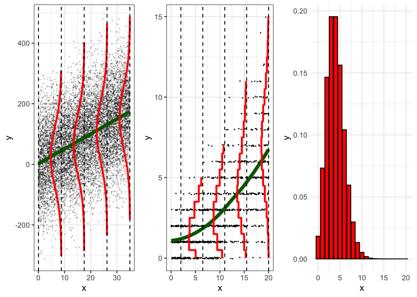
The figure below (adapted from Roback and Legler, 2021) illustrates a comparison of a linear regression model for inference to a Poisson regression using a log function of \(\lambda\).
- The panel on the left shows a linear regression model (in green). Note that the model is linear and that y is normally distributed at different levels of x.
- The middle panel shows the Poisson regression model. The model is non-linear and shows that y follows a Poisson distribution at different levels of x.
- The third panel shows a typical poisson distribution (note that if you flip the middle panel by 90 degrees, the distributions shown reflect the shape from the third panel).
4 Case Study
4.1 What to expect
- In this example the dependent variable is number of days sick, which is a count variable - making Poisson regression an appropriate initial model to test.
- We will learn how to fit Poisson regression models that contain both single and multiple predictors.
- We will also learn how to use residual diagnostic tests to inspect the assumptions of our model.
- Finally, we will learn about overdispersion and how to adjust for this with other models.
4.2 Data Loading and Cleaning
First, we’ll load the HansIll dataset from the speedsR package into our R environment.
# Load the speedsR package
library(speedsR)

# Access and assign the dataset to a variable
Illness <- HansIll
4.3 Exploratory Data Analyses
As always, it is good practice to explore our data descriptively, before we build our models. Much of this has already been covered in Exploratory Data Analysis (EDA) in Sport and Exercise Science, so we will only provide a short example here.
4.3.1 Data organisation
HansIll is a data set that contains 39 variables. Some of the more relevant variables (to this exercise) are listed below:
ID: The participant’s ID numbergroup: The testing condition for the participant, 4x(8x40/20s), 4x(12x40/20s) or 4x8mintime: a binary factor to indicate results for either pre or post testst_symp_score: Total Common Cold symptom scoredays_sick: number of days the participants were sick
Note that for this lesson we will only be using the post-test measurements. As such we should create a filter to only include these measurements (i.e. when time is post). We will also only include the variables of interest in our data set:
Illness_post <- Illness |>
  filter(time == 'post') |>
  dplyr::select('ID', 'group', 'time', 't_symp_score', 'days_sick')
4.3.2 Summary statistics
We can use the skimr package to quickly obtain summary statistics for our chosen variables:
library(skimr)
skim(Illness_post)| Name | Illness_post |
| Number of rows | 25 |
| Number of columns | 5 |
| _______________________ | |
| Column type frequency: | |
| factor | 3 |
| numeric | 2 |
| ________________________ | |
| Group variables | None |
Variable type: factor
| skim_variable | n_missing | complete_rate | ordered | n_unique | top_counts |
|---|---|---|---|---|---|
| ID | 0 | 1 | FALSE | 25 | 1: 1, 2: 1, 4: 1, 5: 1 |
| group | 0 | 1 | FALSE | 3 | 4x(: 9, 4x(: 8, 4x8: 8 |
| time | 0 | 1 | FALSE | 1 | pos: 25, pre: 0 |
Variable type: numeric
| skim_variable | n_missing | complete_rate | mean | sd | p0 | p25 | p50 | p75 | p100 | hist |
|---|---|---|---|---|---|---|---|---|---|---|
| t_symp_score | 0 | 1 | 40.56 | 45.79 | 0 | 8 | 20 | 62 | 184 | ▇▂▂▁▁ |
| days_sick | 0 | 1 | 5.32 | 6.61 | 0 | 0 | 2 | 9 | 20 | ▇▂▂▁▂ |
We can focus on the dependent variable further, by creating a histogram in ggplot:
ggplot(Illness_post, aes(days_sick)) +
  geom_histogram(bins = 10, color = 'white')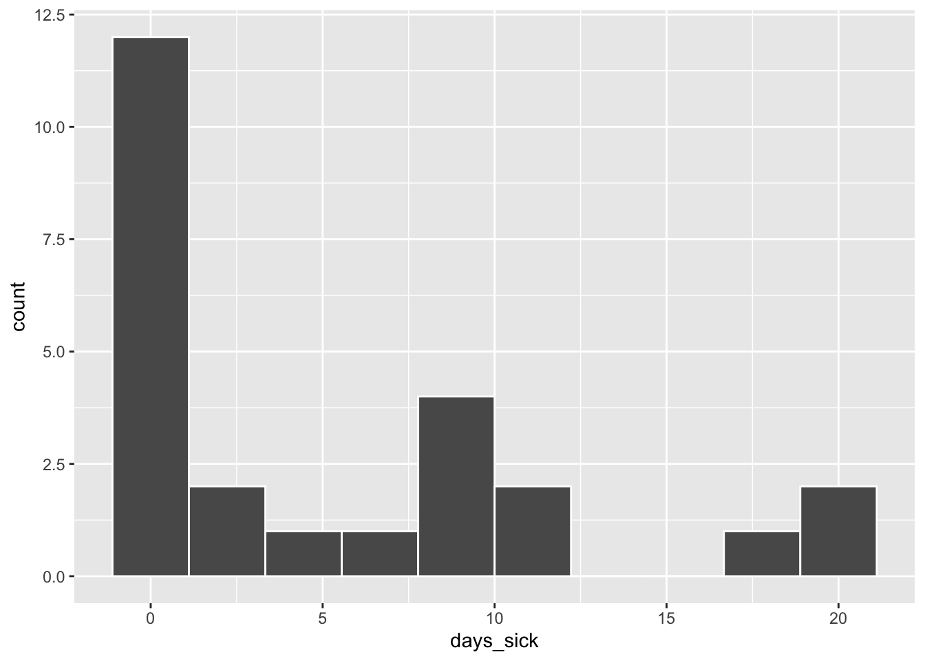
The figure above reveals a fair amount of variability in days sick: responses range from 0 to 20 with most people reporting 0 days sick. The plot is right skewed and clearly indicates that days_sick is not normally distributed.
Important
Note that this many zero’s in the distribution might suggest that a regular Poisson model would not be appropriate either (see Figure 1 to inspect what a Poisson distribution should look like). We will explore this below when we examine over dispersion.
The Poisson regression model also implies that log(\(\lambda_i\)), not the mean days sick \(\lambda_i\), is a linear function of common cold severity score; i.e., \(log(\lambda_i)=\beta_0+\beta_1\textrm{cold score}_i\). Therefore, to check the linearity assumption (Assumption 4) for Poisson regression, we would like to plot log(\(\lambda_i\)) by t_symp_score. Unfortunately, \(\lambda_i\) is unknown. Our best guess of \(\lambda_i\) is the observed mean number of days sick for each common cold score (level of \(X\)). Because these means are computed for observed data, they are referred to as empirical means. Taking the logs of the empirical means and plotting by t_symp_score provides a way to assess the linearity assumption.
sumstats <-
  Illness_post |>
  group_by(t_symp_score) |>
  summarise(m_days_sick = mean(days_sick),
            logm_days_sick = log(m_days_sick))

ggplot(sumstats |> filter(t_symp_score < 180), aes(t_symp_score, logm_days_sick)) +
  geom_point()+
  geom_smooth(method = "loess", size = 1.5) +
  ylab("Log of the empirical mean number of days sick") +
  xlab('Common cold severity score')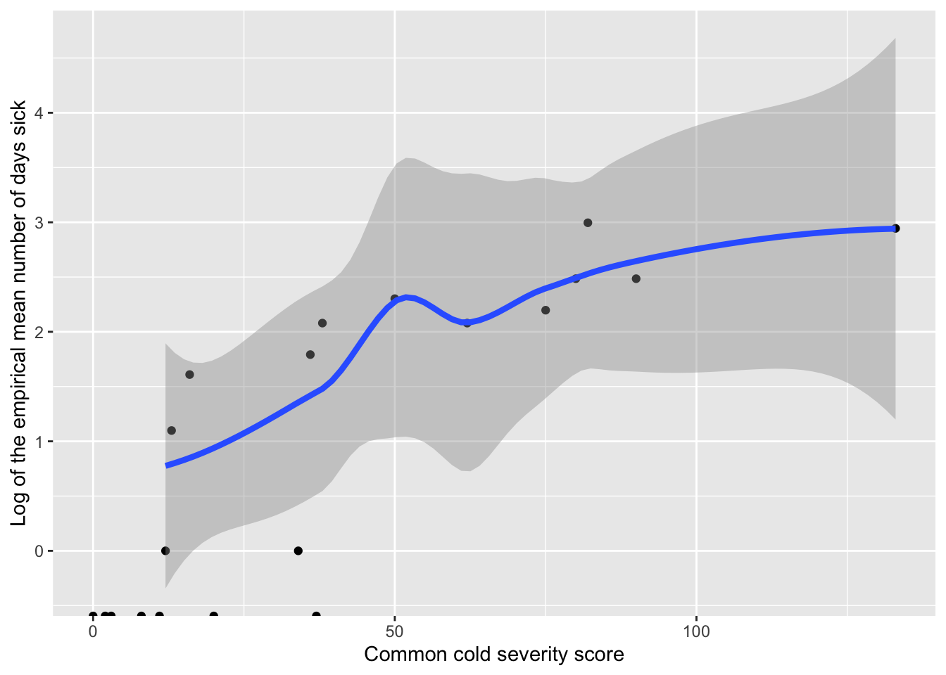
In the plot above, the relationship between cold score and the log of the mean days sick appears relatively linear (note, an extreme outlier has been omitted).
4.4 Estimation and Inference
To begin, we will consider a simple model with only one predictor: t_symp_score. Similar to the linear regression, the estimated regression equation for the Poisson model also contains an intercept (\(\beta_{0}\)) and coefficients for the predictors (\(\beta_{1}\), \(\beta_{2}\), etc.):
\[ log(\hat{\lambda})=\beta_{0}+\beta_{1}x_{1}+\beta_{2}x_{2} + ...+\beta_{n}x_{n} \]
Similar to linear regression, we can use R to obtain the \(\alpha\) and \(\beta\) values. Poisson regression falls under the Generalised Linear Model family, which uses the function glm() to analysis. The code is similar to linear regression, where you have:
- an argument for the formula (in this case:
days_sick~t_symp_score) - an argument for the data (in this case:
Illness_post)
However, in addition to the formula and data, you also need to specify the family, which represents the error distribution and link function to be used in the model. For Poisson regression, the family = ‘Poisson’.
Therefore, we can run a Poisson model in base R with the following:
model1 <- glm(days_sick ~ t_symp_score,
              data = Illness_post,
              family = poisson)
As per usual, we can call the model results with the summary() function:
summary(model1)
Call:
glm(formula = days_sick ~ t_symp_score, family = poisson, data = Illness_post)

Coefficients:
             Estimate Std. Error z value Pr(>|z|)
(Intercept)   0.74564    0.14568   5.118 3.08e-07 ***
t_symp_score  0.01498    0.00131  11.432  < 2e-16 ***
---
Signif. codes:  0 '***' 0.001 '**' 0.01 '*' 0.05 '.' 0.1 ' ' 1

(Dispersion parameter for poisson family taken to be 1)

    Null deviance: 209.539  on 24  degrees of freedom
Residual deviance:  99.806  on 23  degrees of freedom
AIC: 157.68

Number of Fisher Scoring iterations: 5
With this output, we can substitute the Intercept and \(\beta\) coefficient into our model:
\[log(\hat{\lambda})=0.746+0.015t\_symp\_score\]
Note that the equation above would need to be back-transformed to be interpreted in the original units. Here, exponentiating the coefficient on t_symp_score provides us with the multiplicative factor by which the mean count changes.
exp(0.015)[1] 1.015113In this case, the mean number of sick days changes by a factor of \(e^{0.015}=1.015\) or increases by 1.5% with each additional score of Common Cold severity. This is also referred to as a rate ratio or relative risk, and it represents a percent change in the response for a unit change in the predictor.
We can also exponeniate our confidence intervals to interpret them in a similar manner:
exp(confint(model1)) 2.5 % 97.5 %
(Intercept) 1.568051 2.777643
t_symp_score 1.012460 1.017681From the above output, we would be 95% confident that the mean number of sick days increases between 1.25% and 1.77% for each additional score of Common Cold severity. Note that because our interval does not include 1, we can conclude that t_symp_score is significantly associated with number of days sick.
4.4.1 Adding a covariate
Let us now add a covariate to the model, specifically group, which is made up of:
- 4x(8x40/20s),
- 4x(12x40/20s), or
- 4x8min
Recall from the multiple regression lesson that for categorical predictors, a reference level is chosen from the categories, to serve as a baseline for comparison against the other levels. In this example, 4x(12x40/20s) is chosen by default as the reference category.
model2 <- glm(days_sick ~ t_symp_score + group,
              data = Illness_post,
              family = poisson)

summary(model2)
Call:
glm(formula = days_sick ~ t_symp_score + group, family = poisson,
    data = Illness_post)

Coefficients:
                  Estimate Std. Error z value Pr(>|z|)
(Intercept)        0.35632    0.22888   1.557  0.11952
t_symp_score       0.01980    0.00186  10.645  < 2e-16 ***
group4x(8x40/20s)  0.60422    0.21544   2.805  0.00504 **
group4x8min       -0.75589    0.25130  -3.008  0.00263 **
---
Signif. codes:  0 '***' 0.001 '**' 0.01 '*' 0.05 '.' 0.1 ' ' 1

(Dispersion parameter for poisson family taken to be 1)

    Null deviance: 209.54  on 24  degrees of freedom
Residual deviance:  72.48  on 21  degrees of freedom
AIC: 134.35

Number of Fisher Scoring iterations: 6
Like before, we will need to exponeniate the coefficients and confidence intervals to interpret this output:
exp(coef(model2)) (Intercept) t_symp_score group4x(8x40/20s) group4x8min
1.4280704 1.0199927 1.8298202 0.4695931 exp(confint(model2)) 2.5 % 97.5 %
(Intercept) 0.8919344 2.1920425
t_symp_score 1.0163949 1.0238581
group4x(8x40/20s) 1.2037316 2.8074274
group4x8min 0.2845771 0.7645142Note, you can also use the tab_model() function from the sjPlot package to do this for you:
sjPlot::tab_model(model2)
Each of these effects can be interpreted as:
- The mean number of days sick increases by 2% for each additional increase in cold symptom score, and this is statistically significant (95% CI = 1.016 to 1.024, p < .001), when holding other factors constant.
- The mean number of days sick increases by 83% for those in the 4x(8x40/20s) group compared to those in the 4x(12x40/20s) group, and this is statistically significant (95% CI = 1.204 to 2.807, p = .005), when holding other factors constant.
- The mean number of days sick decreases by 53% for those in the [4x8min] group compared to those in the 4x(12x40/20s) group, and this is statistically significant (95% CI = 0.285 to 0.765, p = .003), when holding other factors constant.
As we did with linear regression, we should check the statistical assumptions to have more confidence in our results. To check that these assumptions have been met, we can simply use the check_model() function from the easystats package. Note that the check_model() function provides a range of diagnostic tests. We will only be requesting specific ones for now:
library(easystats)
check_model(model2,
            check = c('overdispersion','outliers','qq','vif'))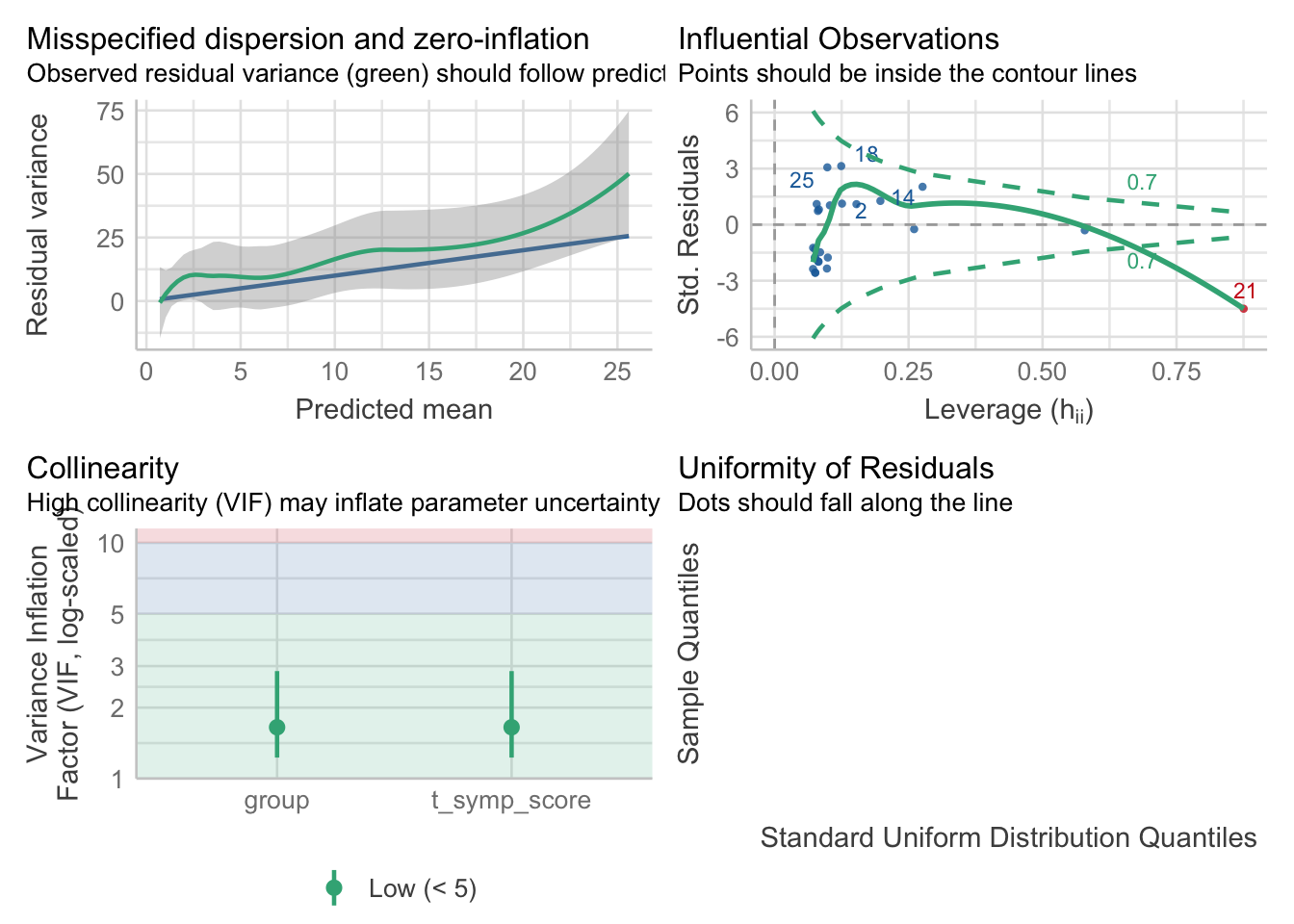
The influential observations, multicollinearity and normality of the residuals plots are interpreted in a similar manner to multiple regression (and this case, these look mostly met, with one influential observation worth investigating).
The assumption of equidispersion is assessed from the top-left panel. If there the mean is approximately equal to the variance, then we would expect a dispersion ratio ~ 1, with the plot displaying the residual variance overlapping the predicted residual variance. Here, the residual variance is greater than the predicted residual variance, as indicated by the green line being above the blue line, at all levels. We can inspect this further with:
check_overdispersion(model2)# Overdispersion test
dispersion ratio = 3.141
Pearson's Chi-Squared = 65.958
p-value = < 0.001The dispersion ratio here is 3.141, with the test indicating that the residual variances being significantly different to the predicted residual variances (\(\chi^{2}=65.96, p < .001\)). Ignoring overdispersion can lead to underestimated standard errors, resulting in overly optimistic inference about the model’s coefficients. Note: we suspected this from the start when we inspected the distribution of sick days.
We will have to try some different models to address this assumption.
4.4.2 Quasi-Poisson Regression
The quasi-Poisson regression model is a flexible extension of the standard Poisson regression that accommodates overdispersion in count data analysis. In quasi-Poisson regression, the variance is allowed to be a multiple of the mean, providing a more realistic representation of the variability in the data. This is achieved by introducing a dispersion parameter that scales the variance, allowing for greater flexibility in modeling count data with varying levels of dispersion. Estimating the dispersion parameter enables adjustment of the standard errors of the coefficient estimates, accounting for the additional variability in the data. Quasi-Poisson regression is particularly useful when dealing with count data exhibiting overdispersion, providing researchers with a robust framework for analyzing data while maintaining the interpretability and simplicity of the Poisson regression model.
It’s quite simple to run a quasi-Poisson model in R. We would just have to change the family type:
model3 <- glm(days_sick ~ t_symp_score + group,
              data = Illness_post,
              family = quasipoisson)
In the table above, we can compare the effects for the two models (Poisson versus Quasi-Poisson). Notice that the Incidence Rate Ratios (exponentiated \(\beta\) coefficients) are the same between the two models. The difference lies in the confidence intervals and the estimation of the p-value. For the Quasi-Poisson Model, only the effect of Cold Symptom Score is statistically significant, with the group comparisons displaying non-significant effects. We should check the assumptions to validate our results:
check_model(model3,
            check = c('overdispersion','outliers','qq','vif'))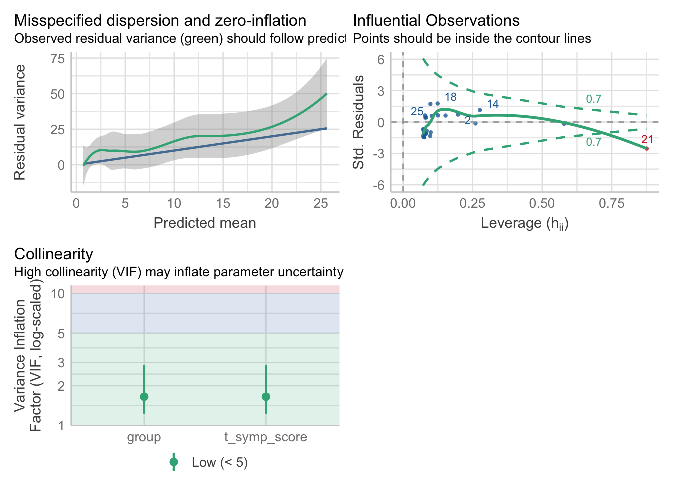
check_overdispersion(model3)# Overdispersion test
dispersion ratio = 3.141
Pearson's Chi-Squared = 65.958
p-value = < 0.001In this case, changing to the quasi-Poisson model only changed to estimates for the confidence intervals, but had little effect on overdispersion. We will have to try a different approach.
4.4.3 Negative Binomial Regression
The negative binomial regression model is a powerful extension of the Poisson regression model designed to handle overdispersed count data. Unlike the Poisson distribution, which assumes that the mean and variance are equal, the negative binomial distribution relaxes this constraint by introducing an additional parameter called the dispersion parameter. This parameter captures the extra variability in the data, allowing the variance to be larger or smaller than the mean. Negative binomial regression estimates both the regression coefficients for predictor variables and the dispersion parameter, providing a flexible and robust approach for modeling count data with overdispersion. By explicitly modeling the variance-mean relationship, negative binomial regression offers improved accuracy in parameter estimation and statistical inference compared to Poisson regression when dealing with overdispersed count data.
While both the negative binomial (NB) regression model and the quasi-Poisson regression model are extensions of the Poisson regression model designed to handle overdispersed count data, they differ in their underlying assumptions and modeling approaches.
- Parameterisation:
- In negative binomial regression, the overdispersion is explicitly modeled through an additional parameter called the dispersion parameter (often denoted as \(\theta\)). This parameter governs the relationship between the mean and variance of the count data.
- In quasi-Poisson regression, overdispersion is addressed by allowing the variance to be a multiple of the mean without directly estimating a dispersion parameter. Instead, the variance is assumed to be proportional to the mean, and the dispersion parameter is implicitly absorbed into the model’s standard errors.
- Flexibility:
- Negative binomial regression provides greater flexibility in modeling the relationship between the mean and variance of count data. The dispersion parameter allows for varying degrees of overdispersion, accommodating cases where the variance is greater or less than the mean.
- Quasi-Poisson regression, while more flexible than the standard Poisson regression, assumes a specific relationship between the mean and variance (i.e., variance is proportional to the mean). This assumption may not always accurately capture the variability in count data, especially in cases where the relationship between the mean and variance is not strictly proportional.
- Interpretation:
- Negative binomial regression estimates both regression coefficients for predictor variables and the dispersion parameter. The interpretation of coefficients remains similar to Poisson regression, while the dispersion parameter quantifies the degree of overdispersion.
- Quasi-Poisson regression does not estimate a dispersion parameter explicitly. Instead, the overdispersion is accounted for through adjusted standard errors of coefficient estimates. Consequently, the interpretation of coefficients in quasi-Poisson regression remains the same as in Poisson regression, with no additional parameter to quantify overdispersion.
The run a negative binomial regression we can use the glm.nb function from the MASS package. Note we do not need to specify the family argument because this is assumed to be negative binomial from the function.
library(MASS)
model4 <- glm.nb(days_sick ~ t_symp_score + group,
                 data = Illness_post)
And like we did before, let us check the assumptions of this new model:
check_overdispersion(model4)# Overdispersion test
dispersion ratio = 1.020
p-value = 0.472Notice that for this model, the dispersion ratio is much closer to 1, and the statistical test has identified no overdispersion.
4.4.4 Zero-Inflated Models
Given the observed distribution of the days_sick variable, where many participants reported zero sick days, it is appropriate to consider zero-inflated models. These models are particularly useful when the data contain an excess of zeros that cannot be adequately modeled by standard Poisson regression. In this section, we will explore how to fit a zero-inflated Poisson (ZIP) model to our data.
4.4.4.1 Understanding Zero-Inflation
Zero-inflated models account for two processes: one that generates the excess zeros and another that represents the count of days_sick among those who experience illness. In our case, we can hypothesise that some participants are inherently healthy (and thus always report zero days sick), while others may experience a count of sick days influenced by factors like symptom severity and group.
4.4.4.2 Fitting a Zero-Inflated Poisson Model
To fit a ZIP model in R, we can use the pscl package, which provides the zeroinfl() function. This function allows us to specify both the count model (which can be a Poisson or negative binomial model) and the zero-inflation model. We can then fit a zero-inflated Poisson model to the data using both t_symp_score and group as predictors in the count model, and we can also include t_symp_score as a predictor for the zero-inflation process.
library(pscl)zip_model <- zeroinfl(days_sick ~ t_symp_score + group | t_symp_score,
data = Illness_post,
dist = "poisson")summary(zip_model)
Call:
zeroinfl(formula = days_sick ~ t_symp_score + group | t_symp_score, data = Illness_post,
    dist = "poisson")

Pearson residuals:
    Min      1Q  Median      3Q     Max
-1.4758 -0.4296 -0.2628  0.4017  1.8871

Count model coefficients (poisson with log link):
                   Estimate Std. Error z value Pr(>|z|)
(Intercept)        1.316248   0.256172   5.138 2.77e-07 ***
t_symp_score       0.012007   0.002099   5.720 1.06e-08 ***
group4x(8x40/20s)  0.274628   0.220482   1.246   0.2129
group4x8min       -0.443564   0.252263  -1.758   0.0787 .

Zero-inflation model coefficients (binomial with logit link):
             Estimate Std. Error z value Pr(>|z|)
(Intercept)   2.41658    1.07019   2.258   0.0239 *
t_symp_score -0.11645    0.05589  -2.084   0.0372 *
---
Signif. codes:  0 '***' 0.001 '**' 0.01 '*' 0.05 '.' 0.1 ' ' 1

Number of iterations in BFGS optimization: 29
Log-likelihood: -43.29 on 6 Df
The output will include coefficients for both the Poisson model and the zero-inflation model. The count model coefficients represent the expected change in the count of sick days, while the zero-inflation model coefficients indicate the predictors associated with the excess zeros. The interpretation for the Count model coefficients is similar to the previous sections. The zero-inflation model coefficients can be interpreted as follows:
Intercept: Estimate = 2.416 This value represents the log-odds of a participant being in the “always zero” group when
t_symp_scoreis at its reference level. The exponentiated value (\(e^{2.416}=11.14\)) indicates that participants with a zero symptom score are 11.14 times more likely to be in the zero group compared to those with higher symptom scores.t_symp_score: Estimate = -0.116 This negative coefficient indicates that as the symptom score increases, the log-odds of being in the “always zero” group decreases. Exponentiating this value (\(e^{-.116}=0.89\)) suggests that for each unit increase in symptom severity, the odds of reporting zero sick days decrease by about 11%. This result is statistically significant (p = 0.0372), indicating that higher symptom scores are associated with a lower likelihood of being in the zero group.
5 Conclusion and Reflection
In conclusion, this guide has provided an overview of regression modeling techniques suitable for count variables, beginning with the assumptions underlying such models. We explored the classical Poisson regression, which assumes equidispersion, and its extensions, including quasi-Poisson and negative binomial regression, which accommodate overdispersion commonly encountered in count data. While our focus was on these three models, it’s worth noting that there are other approaches available, such as zero-inflated and hurdle models, which can further enhance our understanding of count data by addressing excess zeros and modeling zero counts separately from positive counts.
Throughout our discussion, we applied these regression techniques to a practical example of predicting the number of days sick for cyclists, using two predictor variables. However, it’s important to acknowledge that this is just a starting point. We can extend our analysis by incorporating additional predictor variables and we can also explore interactions between variables to uncover more complex relationships and better capture the nuances of the data (see the lesson on Regression Modeling 1).
Further, we could have added random effects (more on this in the multilevel modeling lesson) to account for the repeated measurements in our data. Recall, that we only looked at the post-measurements to avoid violating independence. To include both pre and post, we can fit a generalised linear mixed model (GLMER) to our data:
library(lme4)
glmer_mod <-
  glmer(
    formula = days_sick ~ t_symp_score + group + time + (1|ID),
    data = Illness,
family = poisson)sjPlot::tab_model(model2, model4, glmer_mod,
dv.labels = c('Poisson Model',"Negative Binomial Model", 'GLMER Model'),
collapse.ci = T)| Poisson Model | Negative Binomial Model | GLMER Model | ||||
|---|---|---|---|---|---|---|
| Predictors | Incidence Rate Ratios | p | Incidence Rate Ratios | p | Incidence Rate Ratios | p |
| (Intercept) | 1.43 (0.89 – 2.19) |
0.120 | 0.65 (0.21 – 1.89) |
0.385 | 0.22 (0.04 – 1.15) |
0.073 |
| t symp score | 1.02 (1.02 – 1.02) |
<0.001 | 1.03 (1.02 – 1.04) |
<0.001 | 1.04 (1.02 – 1.05) |
<0.001 |
| group [4x(8x40/20s)] | 1.83 (1.20 – 2.81) |
0.005 | 2.20 (0.79 – 6.31) |
0.142 | 2.61 (0.55 – 12.46) |
0.228 |
| group [4x8min] | 0.47 (0.28 – 0.76) |
0.003 | 1.00 (0.32 – 3.24) |
0.994 | 0.76 (0.15 – 3.88) |
0.740 |
| time [post] | 1.00 (0.79 – 1.27) |
1.000 | ||||
| Random Effects | ||||||
| σ2 | 0.75 | |||||
| τ00 | 1.88 ID | |||||
| ICC | 0.71 | |||||
| N | 25 ID | |||||
| Observations | 25 | 25 | 50 | |||
| R2 Nagelkerke | 0.996 | 0.805 | 0.513 / 0.860 | |||
We won’t go into detail on this output (as it is covered in Lesson 4, and the intention of this was just to provide a demonstration of the procedure). But from the output, we can see that the GLMER model also includes IRRs that can be interpreted in the same manner we have done previously. What GLMER also includes is a component on random effects. This tells us about the variability in the data that is not explained by the fixed effects included in the model. Random effects allow us to account for differences between individual subjects or groups that are not explicitly modeled by the fixed effects. For example, the coefficients associated with our random effect (in this model: participant ID) represent the extent of deviation of each individual from the population average. Positive coefficients indicate that an individual tends to have a higher response than average, while negative coefficients suggest a lower response:
$ID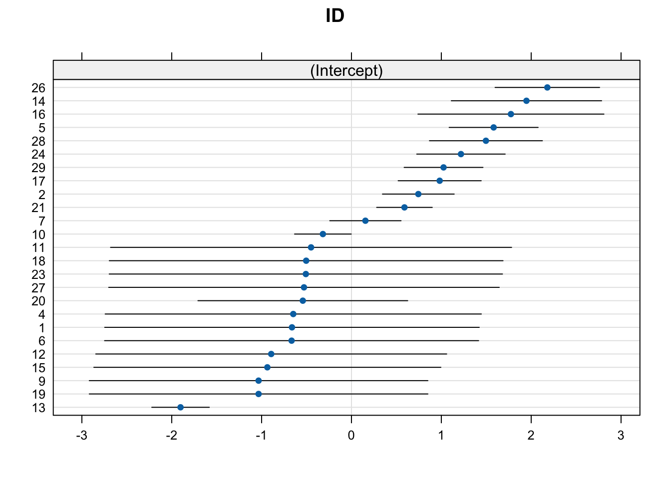
6 Knowledge Spot Check
What type of outcome variable is typically used in Poisson regression?
- Continuous
- Binary
- Count
- Ordinal
- Count
Poisson regression is commonly used when the outcome variable represents counts of events or occurrences, such as the number of accidents, the number of deaths, or the number of customer arrivals. It assumes that the outcome variable follows a Poisson distribution, which is appropriate for count data.
In Poisson regression, what is the link function commonly used to model the relationship between the predictor variables and the mean of the outcome variable?
- Identity function
- Logit function
- Exponential function
- Log function
- Log function
The log function (also known as the logarithmic or log-link function) is commonly used in Poisson regression to model the relationship between the predictor variables and the mean of the outcome variable. It ensures that the predicted values of the outcome variable are non-negative and interpretable on the log scale.
When interpreting the incidence rate ratios (IRRs) in Poisson regression, what does an IRR greater than 1 indicate?
- The expected count of the outcome variable decreases by the value of the IRR for a one-unit increase in the predictor variable.
- The expected count of the outcome variable increases by the value of the IRR for a one-unit increase in the predictor variable.
- There is no relationship between the predictor variable and the expected count of the outcome variable.
- The IRR cannot be interpreted in Poisson regression.
- The expected count of the outcome variable increases by the value of the IRR for a one-unit increase in the predictor variable.
In Poisson regression, the incidence rate ratio (IRR) quantifies the change in the expected count of the outcome variable for a one-unit increase in the predictor variable. An IRR greater than 1 indicates that the expected count of the outcome variable increases by the value of the IRR for each one-unit increase in the predictor variable. This implies a positive association between the predictor variable and the outcome variable’s count.
What does overdispersion indicate in the context of Poisson regression?
- The variability of the outcome variable is less than expected based on the Poisson distribution.
- The variability of the outcome variable is greater than expected based on the Poisson distribution.
- The outcome variable follows a normal distribution rather than a Poisson distribution.
- The outcome variable is perfectly predicted by the predictor variables.
- The variability of the outcome variable is greater than expected based on the Poisson distribution.
Overdispersion in Poisson regression occurs when the observed variability of the outcome variable is larger than what would be expected under the assumption of a Poisson distribution. This means that there is more variability in the data than can be accounted for by the model, which may lead to incorrect standard errors and inflated Type I error rates if not addressed appropriately.
How does overdispersion affect the standard errors and hypothesis testing in Poisson regression?
- Overdispersion has no effect on standard errors and hypothesis testing.
- Overdispersion inflates standard errors, leading to underestimated p-values and potentially misleading inference.
- Overdispersion reduces standard errors, leading to overly conservative p-values and less sensitive hypothesis testing.
- Overdispersion results in more accurate standard errors and hypothesis testing due to increased variability.
- Overdispersion inflates standard errors, leading to underestimated p-values and potentially misleading inference.
In Poisson regression, overdispersion can inflate the standard errors of the estimated coefficients, making them larger than they should be under the assumption of a Poisson distribution. This inflation of standard errors results in underestimated p-values, which can lead to incorrect conclusions about the significance of predictor variables. Therefore, overdispersion can compromise the validity of hypothesis testing in Poisson regression if not properly addressed.