rm(list = ls()) # clear the workspace

# Libraries required for data manipulation
library(dplyr) # provides functions for manipulating datasets
library(ggplot2) # provides functions for data visualizations
library(stringr) # simplifies the process of working with strings, providing consistent and easy-to-understand functions
library(visdat) # enables visual inspection of data quality and structure
library(speedsR) # collection of sports-specific benchmark datasets - part of the AIS SPEEDS project

# Loading datasets directly from the `speedsR` package
dataset_names <- c("cycling_untidy_fictitious_data_1",
                   "cycling_untidy_fictitious_data_2",
                   "cycling_untidy_fictitious_data_3",
                   "cycling_untidy_fictitious_data_4",
                   "cycling_untidy_fictitious_data_5")

# Concatenating datasets into a single tibble
cycling_data <- bind_rows(lapply(dataset_names, function(name) get(name)))Data Integrity: Handling Missing Data and Outliers
Handling and Mitigating the Impact of Missing Data and Outliers in Sports Data Analysis
Abstract
Explore the critical aspects of maintaining data integrity in sports and exercise science through proficient handling of missing data and outliers. This lesson guides you through identifying, understanding, and addressing these data challenges, using R to implement strategies that enhance dataset quality and reliability. Learn to apply deletion and imputation techniques for missing data and discover methods to identify and manage outliers, ensuring your data analysis is accurate and insightful. Tailored for sports analysts and data practitioners, this lesson empowers you with the skills to refine sports data, transforming potential data integrity issues into opportunities for deeper analysis and informed decision-making. Whether you’re assessing athlete performance or optimizing training programs, mastering these techniques is essential for data-driven sports science.
Keywords
Data Integrity, Sports Analytics, Missing Data, Outliers, Data Cleaning, Data Imputation, Data Visualization, R Programming, Exploratory Data Analysis (EDA), Boxplot, Scatter Plot, Mean, Median, Interquartile Range (IQR), dplyr, ggplot2, visdat, speedsR.
Lesson’s Level
The level of this lesson is categorized as BRONZE.
Lesson’s Main Idea
- Ensuring data integrity through effective management of missing data and outliers is crucial in sport and exercise science analytics, ensuring analyses are based on accurate and comprehensive information.
- The lesson introduces practical strategies and R tools for handling missing data and outliers, including deletion, imputation, and visualization techniques, equipping practitioners with methods to enhance data reliability and analysis quality.
Dataset Featured In This Lesson
Disclaimer: The dataset featured in this lesson is entirely fictitious and has been artificially created for pedagogical purposes. Any resemblance to actual persons, living or deceased, or real-world data is purely coincidental and not intended.
1 Learning Outcomes
By the end of this lesson, you will have developed the skills to:
Identify and Understand Missing Data: Recognize the different types of missing data within sports and exercise science datasets and comprehend their implications on data analysis.
Apply Strategies for Handling Missing Data: Employ practical methods to address missing data, including deletion and imputation techniques, leveraging R’s capabilities to maintain or restore dataset integrity.
Visualize and Identify Outliers: Utilize visualization tools to detect outliers in the data, gaining insights into their nature and potential impact on sports analytics.
Implement Outlier Management Techniques: Choose and apply appropriate strategies for managing outliers, considering the context and objectives of the analysis, to enhance the reliability of conclusions drawn from the data.
2 Introduction: Ensuring Data Integrity in Sport and Exercise Science
In the field of sports and exercise science, data serves as the cornerstone for making informed decisions that enhance athlete performance and optimize training programs. However, the utility of this data is heavily dependent on its quality — its completeness and accuracy. Missing data and outliers can significantly compromise data integrity, leading to flawed analyses and potentially misleading conclusions. This lesson explores the critical aspects of handling missing data and outliers, emphasizing their impact on sports analytics.
2.1 The Challenge of Missing Data and Outliers
Missing data occurs when no value is stored for a variable within a dataset, often indicated as N/A, NaN, or simply left blank. Outliers, on the other hand, are data points that deviate significantly from other observations. Both present unique challenges in data analysis, particularly in sports analytics, where precise measurements are crucial for performance assessment and strategic planning.
2.1.1 Why It’s Important to Handle Missing Data
The presence of missing data undermines the reliability of a dataset, creating gaps in information that can distort the understanding of an athlete’s performance or a team’s dynamics. Effectively handling missing data is essential to maintain statistical power and ensure accurate, evidence-based conclusions. In sports analytics, where datasets often describe populations of athletes or events, addressing missing data enables a comprehensive analysis of performance trends and health metrics.
2.1.2 Why Data Might Be Missing
Missing data can result from a variety of causes, from systematic errors during data collection to the absence of information provided by data sources. Identifying the underlying reasons for missing data is the first step in determining the most appropriate method for addressing it.
The most common reason for missing data is the failure to record a value for a variable. This omission can occur at any stage of the data collection process, whether due to technological issues or human error. Understanding these systematic causes is crucial for preventing missing data and ensuring dataset completeness.
2.1.3 Identifying and Checking for Missing Data
To safeguard against the implications of missing data, it’s vital to employ strategies for its identification and resolution:
Verifying Data Uploads: Ensuring data is accurately uploaded from the outset can prevent missing data due to technical glitches.
Inspecting Data Samples: Examining small portions of the dataset can help quickly identify missing values.
Utilizing Summary Statistics: Generating summary statistics for the dataset can highlight discrepancies in data counts, signaling the presence of missing data.
The process of handling missing data in sport and exercise science involves a careful assessment of the dataset’s scope and the potential impact of any missing values. By applying appropriate strategies — from data imputation to deletion of incomplete entries — researchers and practitioners can preserve the integrity of their analyses, drawing insights that are both accurate and actionable. This foundational understanding sets the stage for exploring specific techniques and considerations in managing missing data and outliers within the sports analytics domain.
3 Understanding Missing Data
In the domain of sport and exercise science, data integrity plays a crucial role. This section delves into the types of missing data, each characterized by its pattern of missingness, and provides sport-specific examples to illustrate how such situations can arise in practice.
3.1 Types of Missing Data
Data missingness can significantly impact the conclusions drawn from a study or analysis. It is vital to understand the nature of missing data to apply the most appropriate handling methods. Missing data can be broadly categorized into three types: Missing Completely at Random (MCAR), Missing at Random (MAR), and Missing Not at Random (MNAR).
3.1.1 Missing Completely at Random (MCAR)
In MCAR, the likelihood of data being missing is uniform across all observations. An example in sport and exercise science might be a situation where a fitness tracking device sporadically fails to record the heart rate during a training session due to technical glitches, affecting data entries randomly.
| Participant ID | Activity Type | Heart Rate (bpm) |
|---|---|---|
| 1 | Running | 150 |
| 2 | Cycling | |
| 3 | Swimming | 140 |
| 4 | Running | |
| 5 | Cycling | 160 |
This example illustrates random missingness in heart rate data due to device failure, not related to any specific condition of the participants or the type of activity.
3.1.2 Missing at Random (MAR)
MAR occurs when the propensity for data to be missing is related to observed data but not to the missing data itself. For instance, younger athletes might be less diligent in recording their dietary intake, making the missingness dependent on the observed data (age) but not on the dietary intake itself.
| Participant ID | Age | Dietary Intake (calories) |
|---|---|---|
| 1 | 18 | |
| 2 | 25 | 2500 |
| 3 | 30 | 2300 |
| 4 | 19 | |
| 5 | 27 | 2200 |
The pattern of missing dietary intake data among younger athletes illustrates MAR, where missingness is related to age, an observed variable.
3.1.3 Missing Not at Random (MNAR)
MNAR happens when the missingness is related to the unobserved data itself. A relevant scenario in sport and exercise science could involve athletes with injuries being less inclined to report their performance metrics, fearing that the data might reflect poorly on their capabilities.
| Participant ID | Injury Status | Performance Score |
|---|---|---|
| 1 | None | 85 |
| 2 | Minor | |
| 3 | None | 90 |
| 4 | Major | |
| 5 | None | 88 |
In this case, the absence of performance scores for injured athletes signifies MNAR, as the missingness directly correlates with the undisclosed poor performance related to their injuries.
Understanding these categories of missing data facilitates the development of targeted strategies for their management, crucial for maintaining the quality and reliability of data analyses in sport and exercise science. Each type requires a nuanced approach, from imputation methods tailored for MCAR situations to more sophisticated techniques for addressing MAR and MNAR, ensuring the integrity of research findings and applications in the field.
3.2 Exploring Data Missingness In Your Dataset
After discussing the types and impacts of missing data in sport and exercise science, this subsection moves to practical exploration. Using a fictitious cycling dataset from the speedsR package, we’ll show how to identify and visualize missing data, leveraging the concatenated dataset cycling_data. This demonstration is crucial for preparing the data for in-depth analysis and ensuring that subsequent decisions are informed by accurate and comprehensive information. Through a streamlined process in R, we aim to uncover the presence and patterns of missing data, equipping you with the knowledge to implement effective strategies for addressing these issues.
3.2.1 Loading and Preparing Data for Analysis
To explore data missingness, we start by accessing an array of fictitious datasets designed for educational purposes, provided through the speedsR package. These datasets, while synthetic, replicate the complex scenarios often faced by practitioners in sport and exercise science, making them ideal for our exploration.
This streamlined process creates a comprehensive dataset, cycling_data, ready for the analysis in this lesson. By combining datasets in this manner, we mimic the real-world scenario of working with extensive and multifaceted data, characteristic of the sport and exercise science field.
3.2.2 Preliminary Data Cleaning Steps
Before diving into exploring missingness, it’s essential to ensure our dataset is properly cleaned and prepared. The following steps are crucial for standardizing the dataset, making it easier to work with and analyze. Detailed explanations of these steps can be found in our dedicated lesson on Data Cleaning and Wrangling.
3.2.2.1 Initial Data Exploration
# Display the first few rows of the dataset
head(cycling_data)
# A tibble: 6 × 8
ID Race_date Team participant `Gender AGE` `heart RATE` `DISTANCE km`
<int> <chr> <chr> <chr> <chr> <dbl> <dbl>
1 1 07-06-2023 Victoria… Mary_White <NA> NA 36.5
2 2 15-11-2023 Queensla… Elizabeth_… F33 146 66.3
3 3 11-06-2023 Tasmania… Robert_Smi… M18 73 90.6
4 4 <NA> <NA> Jennifer_W… F25 123 NA
5 5 18-07-2023 Tasmania… Mary_Jones F19 69 88.1
6 6 20-02-2023 Queensla… Mary_Smith F30 67 49.1
# ℹ 1 more variable: `VO2 MAX` <chr># Get a statistical summary of the dataset
summary(cycling_data) ID Race_date Team participant
Min. : 1.0 Length:35 Length:35 Length:35
1st Qu.: 9.5 Class :character Class :character Class :character
Median :18.0 Mode :character Mode :character Mode :character
Mean :18.0
3rd Qu.:26.5
Max. :35.0
Gender AGE heart RATE DISTANCE km VO2 MAX
Length:35 Min. : 60.00 Min. :31.44 Length:35
Class :character 1st Qu.: 89.75 1st Qu.:48.84 Class :character
Mode :character Median :115.00 Median :71.23 Mode :character
Mean :113.67 Mean :67.75
3rd Qu.:139.50 3rd Qu.:83.21
Max. :175.00 Max. :97.06
NA's :5 NA's :7 # Find out the number of rows in the dataset
nrow_cycling_data <- nrow(cycling_data)3.2.2.2 Cleaning Column Names
# Retrieve and clean column names for consistency and ease of use
col_names <- colnames(cycling_data) %>%
  tolower() %>%
  gsub("^\\s+|\\s+$", "", .) %>%
  gsub(" ", "_", .)

# Apply the cleaned column names back to the dataset
colnames(cycling_data) <- col_names

# Manually rename specific columns for clarity
cycling_data <- rename(cycling_data, VO2_max = vo2_max, ID = id)
3.2.3 Investigating Missingness
With the dataset cleaned and column names standardized, we now focus on identifying and visualizing the missing data within cycling_data.
3.2.3.1 Identifying and Addressing Empty Cells
First, we convert any empty cells to NA, standardizing the representation of missing values across the dataset.
# Replace empty cells with NA
cycling_data[cycling_data == ""] <- NA
3.2.3.2 Counting Missing Values
To assess the extent of missing data, we count the missing values in each column and the dataset as a whole.
# Count the number of NA values in each column
NA_count_per_column <- sapply(cycling_data, function(x) sum(is.na(x)))
print(NA_count_per_column)
ID race_date team participant gender_age heart_rate
0 6 6 0 5 5
distance_km VO2_max
7 4 # Compute the total number of missing values in the dataset
total_NA_count <- sum(is.na(cycling_data))
print(total_NA_count)[1] 333.2.3.3 Visualizing Missing Data
Lastly, we use the vis_miss() function from the visdat package to visually inspect the distribution of missing data within our dataset.
# Visualize missing data
vis_miss(cycling_data)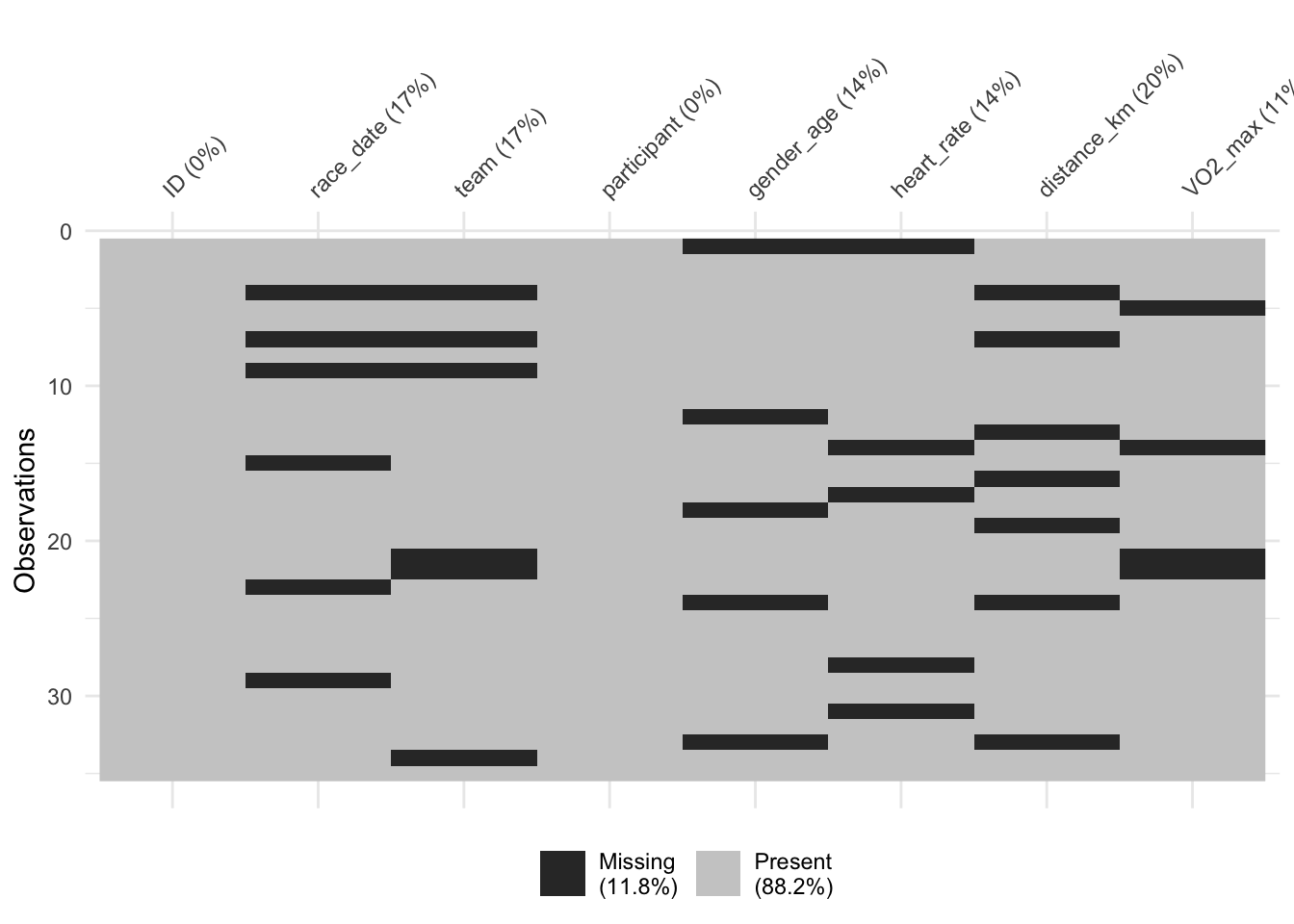
This visualization step not only reveals the presence of missing data but also patterns that may indicate whether the data is Missing Completely at Random (MCAR), Missing at Random (MAR), or Missing Not at Random (MNAR). Such insights are invaluable, guiding us in selecting the most appropriate techniques for handling missingness, whether through imputation, deletion, or more complex statistical modeling approaches.
4 Approaches for Handling Missing Data
Now that we’ve identified and visualized missing data in our dataset, understanding its nature and implications, the next critical step is to select an optimal strategy for addressing this missingness, ensuring the dataset’s integrity remains intact. Handling missing data effectively is paramount in sports data analysis, as it allows for a more accurate and comprehensive understanding of athletes’ performance, health metrics, and other vital statistics. This section delves into various strategies for managing missing data, focusing on deletion and imputation techniques. We’ll explore how these approaches can be applied in sports data analysis, highlighting specific tools in R suited for these tasks and advising on the most appropriate methods based on the type of missing data encountered.
4.1 Handling Missing Data With Deletion - Use With Caution
Handling missing data with deletion is a strategy that comes with inherent risks and should be approached with caution. This method involves removing records or features from your dataset that contain missing values, through either listwise (complete-case) deletion or pairwise deletion.
Listwise Deletion: This approach removes entire records from the dataset if any single value is missing. It’s simple and can be easily implemented but may lead to significant data loss, especially if the dataset contains a lot of missing values. This method assumes that the missing data is Missing Completely at Random (MCAR), which may not always be the case.
Pairwise Deletion: Used mainly in statistical analysis, pairwise deletion allows the use of available data by analyzing pairs of variables without discarding entire records. It’s more data-efficient than listwise deletion but can introduce bias if the assumption of data being MCAR is violated.
4.1.1 Precautions When Using Deletion
While deletion methods can be useful, they come with precautions:
Data Loss: Both listwise and pairwise deletions can result in a substantial amount of data being discarded, which may reduce the statistical power of any analysis conducted on the dataset.
Bias: If the missing data is not MCAR, deletion methods can introduce bias into the analysis, leading to inaccurate conclusions.
Because of these potential drawbacks, deletion should be considered carefully. It may be suitable for datasets where the proportion of missing data is minimal and is believed to be MCAR. However, in many cases, especially when dealing with larger amounts of missing data or when the data is not MCAR, alternative strategies such as imputation might be more appropriate to preserve the integrity and usefulness of the dataset.
4.2 Handling Missing Data - Imputation Techniques
Building on our exploration of missing data, we delve into effective imputation strategies that offer a structured approach to addressing gaps within sports and exercise science datasets. Highlighted here are key techniques including Mean/Median/Mode Imputation, K-Nearest Neighbors (KNN) Imputation, and Multiple Imputation by Chained Equations (MICE), which incorporates Predictive Mean Matching (PMM) for nuanced imputation. Each method is evaluated for its applicability and effectiveness in various scenarios, providing a comprehensive toolkit for maintaining dataset integrity.
4.2.1 Mean/Median/Mode Imputation
How it Works: This technique imputes missing values using the central tendency of the data — mean for numeric data, median for skewed numeric data, and mode for categorical data. It is particularly suitable for data missing completely at random (MCAR), providing a straightforward and effective approach to maintaining the integrity of sports and exercise science datasets. The implementation in R is facilitated by the dplyr package, making it an accessible option for sport science practitioners.
When to Use: Best for data Missing Completely At Random (MCAR) where the absence of data is independent of any variables. For example, if data from a fitness tracker is sporadically missing due to device error, the missing values can be imputed with this method.
Suitable for Types of Missing Data: MCAR.
4.2.2 K-Nearest Neighbors (KNN) Imputation
How it Works: KNN Imputation identifies the ‘k’ closest neighbors within the observed data based on the similarity of available features to fill in missing values. This proximity is determined by the distance between data points, offering a nuanced approach that goes beyond simple averages.
When to Use: Particularly beneficial for MAR situations, where the pattern of missingness is related to observable data. An example includes predicting missing nutritional data for athletes during off-seasons by analyzing similar periods with complete information.
Suitable for Types of Missing Data: Optimally used for MAR data, as it relies on the relationships within the observed parts of the dataset to estimate missing values.
4.2.3 Multiple Imputation by Chained Equations (MICE) with Predictive Mean Matching (PMM)
How it Works: MICE addresses missing data by generating multiple imputed datasets, thus reflecting the inherent uncertainty. Through a series of regression models, each tailored to variables with missing entries, it offers a comprehensive approach to imputation. PMM, a key technique within MICE, enhances this process by selecting observed values close to the predicted values for the missing data, useful for handling skewness or outliers.
When to Use: This method shines when dealing with complex missing data scenarios, including MAR and MNAR, by leveraging the full dataset for more accurate imputation. It’s particularly valuable for nuanced cases, such as underreported training data among athletes.
Suitable for Types of Missing Data: Designed to effectively tackle both MAR and MNAR data, making it a versatile option in sports and exercise science analysis where data missingness can be multifaceted.
For a detailed example of missing data imputation with MICE and PMM, refer to our lesson on synthetic data generation Synthetic Data Generation.
| Technique | Data Suitability | Use Case Example |
|---|---|---|
| Mean/Median/Mode | MCAR | Missing data from a fitness tracker due to device error |
| K-Nearest Neighbors | MAR | Missing nutritional data during off-season based on patterns from complete data |
| MICE (with PMM) | MAR, MNAR | Skilled athletes’ incomplete training logs |
These techniques offer a range of options for handling missing data in sport and exercise science, from simple approaches suitable for randomly missing data to more sophisticated methods that account for complex missing data patterns. The choice of technique should be guided by the nature of the missing data, the structure of the dataset, and the specific requirements of the analysis.
4.3 Common Pitfalls in Handling Missing Data
In tackling missing data, it’s crucial to steer clear of overly simplistic fixes. Replacing missing values with zeros or just deleting them might seem easy but can significantly bias your analysis. This is particularly true when zero values themselves can be meaningful or represent actual observations in sports and exercise science data. Misusing zeros as placeholders for missing data can distort the true picture your data presents, affecting the outcomes of exploratory data analysis (EDA) and subsequent conclusions. Remember, discerning the actual meaning of zeros in your dataset is key to accurate and insightful analysis.
5 Understanding and Handling Outliers
After exploring the intricacies of missing data in sport and exercise science datasets, our journey continues with understanding outliers — those extreme observations that stand apart from the rest. Outliers can significantly influence the analysis and interpretation of data, making it crucial to identify and understand them. Whether these outliers signal data entry errors, unique events, or natural variability, recognizing their presence and nature is vital. In sports and exercise science, outliers might represent extraordinary performances or unusual measurements that could skew analysis if not properly accounted for.
5.1 Types of Outliers
5.1.1 Global Outliers
Point outliers are individual data points that diverge significantly from the rest of the data. For example, consider the recorded maximum oxygen uptake (VO2 max) values for a group of athletes, where one athlete’s value is abnormally high due to a data entry error or an exceptional physiological condition. Identifying such outliers is essential to ensure they do not distort the analysis.
5.1.2 Contextual Outliers
These outliers depend on the specific context of the data. For instance, a runner’s significantly faster lap time during a training session might be an outlier if it occurs under unusual weather conditions or on a different track surface. Contextual outliers require a nuanced approach, as they might only be considered outliers under certain conditions.
5.1.3 Collective Outliers
When a group of data points deviates from the overall pattern, they are termed collective outliers. An example within sports could be a series of performance metrics for a team that suddenly improves over a short period, possibly due to changes in training techniques or team composition. Such outliers might indicate a shift in the underlying process or condition being measured.
5.2 Considerations For Handling Outliers
Identifying outliers is a critical step, but deciding how to handle them requires careful consideration. Visualization tools can be instrumental in spotting unusual patterns or values in the data. The decision to remove or adjust outliers should always be made with the dataset’s context and the analysis goals in mind, ensuring that any modifications do not compromise the data’s integrity or the analysis’s objectivity.
For example, removing the data of an exceptionally skilled athlete might simplify the overall analysis but would omit valuable insights into the potential for human performance. Similarly, adjusting values to account for identifiable and explainable variations (like weather conditions affecting performance) can help refine the analysis without losing the richness of the data.
5.3 Identifying Outliers in Heart Rate Data (Example)
In this part of our lesson on managing outliers, we’ll use the cycling_data dataset to illustrate how outliers can be identified, particularly within the heart_rate column. Our goal is to enrich our dataset with a practical example, thereby enhancing our understanding of outlier detection techniques.
5.3.1 Artificially Adding High Outliers to the Dataset
To demonstrate outliers in heart_rate, we’ll introduce two artificially high values into our dataset. This R code snippet accomplishes this by appending new rows with outlier values:
# Adding outliers to the heart_rate column
outlier_entries <- data.frame(
  ID = c(max(cycling_data$ID) + 1, max(cycling_data$ID) + 2),
  race_date = c(NA, NA),
  team = c(NA, NA),
  participant = c("Outlier_1", "Outlier_2"),
  gender_age = c(NA, NA),
  heart_rate = c(230, 260), # Artificially high outliers for demonstration purposes
  distance_km = c(NA, NA),
  VO2_max = c(NA, NA)
)

# Inserting outliers into the cycling_data dataset randomly
set.seed(123) # Ensuring reproducibility
random_rows <- sample(1:nrow(cycling_data), 2)
cycling_data <- rbind(cycling_data, outlier_entries)
5.3.2 Analyzing Mean and Median
Understanding the central tendencies of heart_rate can hint at the data distribution’s skewness. Calculating and comparing the mean and median heart rates:
mean_heart_rate <- mean(cycling_data$heart_rate, na.rm = TRUE)
median_heart_rate <- median(cycling_data$heart_rate, na.rm = TRUE)

print(paste("Mean heart rate:", mean_heart_rate))
[1] "Mean heart rate: 121.875"print(paste("Median heart rate:", median_heart_rate))[1] "Median heart rate: 120"Observing that the mean is higher than the median suggests a right-skewed distribution, indicating the presence of outliers. This skewness indicates that there are outliers present on the higher end of the dataset. The presence of such outliers can pull the mean upwards, making it larger than the median, which is more resistant to extreme values. In the context of the heart_rate data, this would mean that there are values significantly higher than the majority of the data, hinting at the presence of outliers on the higher side of the heart rate measurements.
5.3.3 Visualizing Outliers with a Boxplot
Let’s visualize the heart rate distribution with a boxplot that will help us identify outliers:
boxplot(cycling_data$heart_rate,
        main = "Heart Rate Distribution",
        ylab = "Heart Rate (bpm)",
        col = "lightblue",
        notch = FALSE) # Notches indicate the confidence interval around the median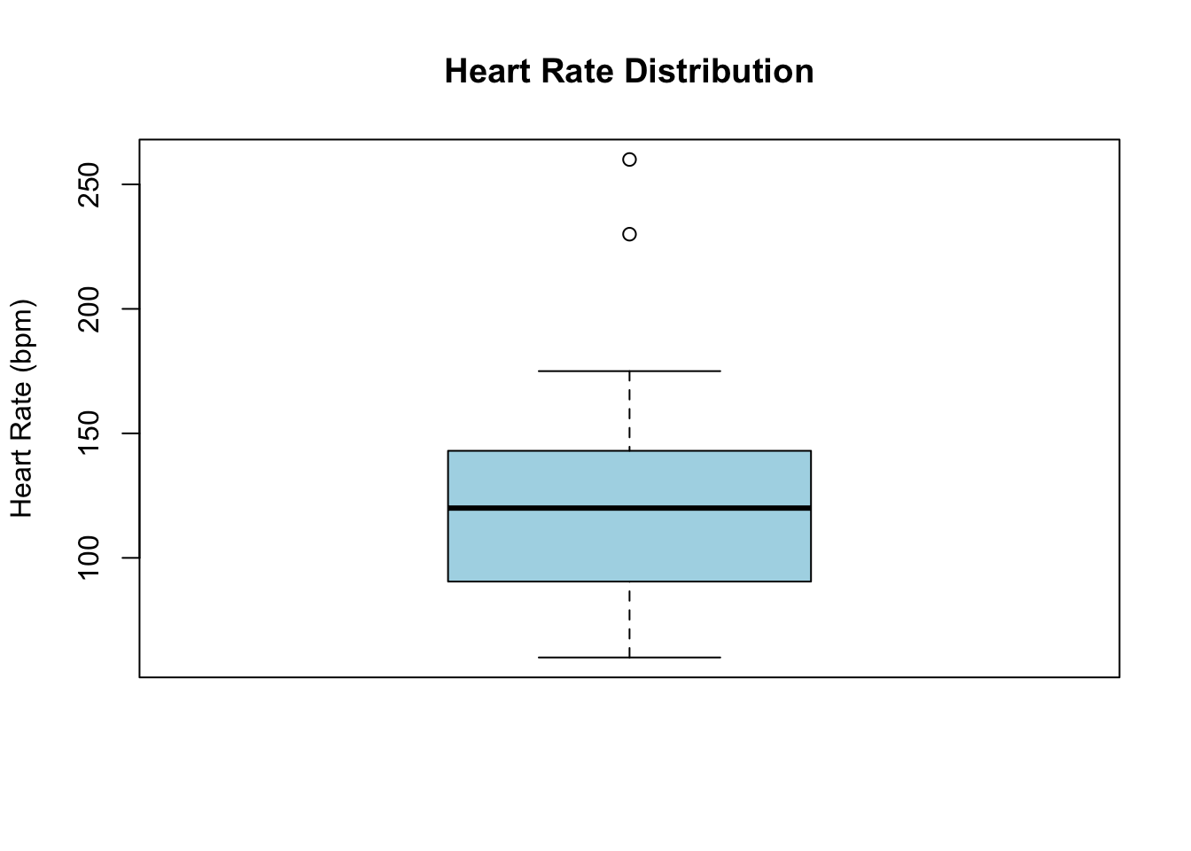
This plot clearly shows our artificially added outliers beyond the box plot whiskers, emphasizing their deviation from the typical range of data.
5.3.4 Calculating the Interquartile Range (IQR) and Defining Outliers
To precisely identify outliers, we calculate the Interquartile Range (IQR), a critical measure in statistics representing the spread of the middle 50% of the data values. The IQR is computed as the difference between the third quartile (Q3) and the first quartile (Q1) of the dataset:
Q1 <- quantile(cycling_data$heart_rate, 0.25, na.rm = TRUE)
Q3 <- quantile(cycling_data$heart_rate, 0.75, na.rm = TRUE)
IQR <- Q3 - Q1
The IQR focuses on the central portion of the dataset and is depicted by the length of the box in a boxplot. It helps us determine the variability within the data’s middle 50%, setting the stage to identify outliers effectively:
upper_limit <- Q3 + 1.5 * IQR
lower_limit <- Q1 - 1.5 * IQR

print(paste("Q1 (25th percentile):", Q1))
[1] "Q1 (25th percentile): 91.25"print(paste("Q3 (75th percentile):", Q3))[1] "Q3 (75th percentile): 141.5"print(paste("Interquartile Range (IQR):", IQR))[1] "Interquartile Range (IQR): 50.25"print(paste("Upper Limit:", upper_limit))[1] "Upper Limit: 216.875"print(paste("Lower Limit:", lower_limit))[1] "Lower Limit: 15.875"In statistical practice, any data point lying more than 1.5 times the IQR above the third quartile (Q3) or below the first quartile (Q1) is considered an outlier. These are the points that appear beyond the whiskers in a boxplot. However, it’s essential for data professionals to exercise caution; an outlier isn’t necessarily an error. Outliers may represent valuable information about the dataset’s behavior or indicate special cases that warrant further investigation.
5.3.5 Identifying Outliers with Boolean Masks
After establishing the upper and lower limits for what constitutes an outlier in the heart_rate data, we can isolate these outliers using a Boolean mask. This technique allows us to filter and examine the data points that fall outside the typical range:
# Boolean mask for outliers
outliers_mask <- with(cycling_data, heart_rate < lower_limit | heart_rate > upper_limit)

# Selecting outliers
outliers <- cycling_data[outliers_mask, ]
print("Outliers based on heart rate:")
[1] "Outliers based on heart rate:"print(outliers)# A tibble: 7 × 8
ID race_date team participant gender_age heart_rate distance_km VO2_max
<dbl> <chr> <chr> <chr> <chr> <dbl> <dbl> <chr>
1 NA <NA> <NA> <NA> <NA> NA NA <NA>
2 NA <NA> <NA> <NA> <NA> NA NA <NA>
3 NA <NA> <NA> <NA> <NA> NA NA <NA>
4 NA <NA> <NA> <NA> <NA> NA NA <NA>
5 NA <NA> <NA> <NA> <NA> NA NA <NA>
6 36 <NA> <NA> Outlier_1 <NA> 230 NA <NA>
7 37 <NA> <NA> Outlier_2 <NA> 260 NA <NA> This code displays the rows from cycling_data where heart_rate values fall below the lower limit or above the upper limit, effectively identifying the outliers.
5.3.6 Visualizing Outliers with a Scatter Plot
Visualizing our data, including the outliers, can provide deeper insights into their distribution and impact. A scatter plot is an effective way to achieve this:
# Scatter plot for heart_rate with outliers highlighted
ggplot(cycling_data, aes(x = ID, y = heart_rate)) +
  geom_point(aes(color = heart_rate < lower_limit | heart_rate > upper_limit), size = 2) +
  scale_color_manual(values = c("TRUE" = "red", "FALSE" = "black")) +
  labs(title = "Heart Rate Outliers", x = "Participant ID", y = "Heart Rate (bpm)") +
  theme_minimal() +
  theme(legend.title = element_blank())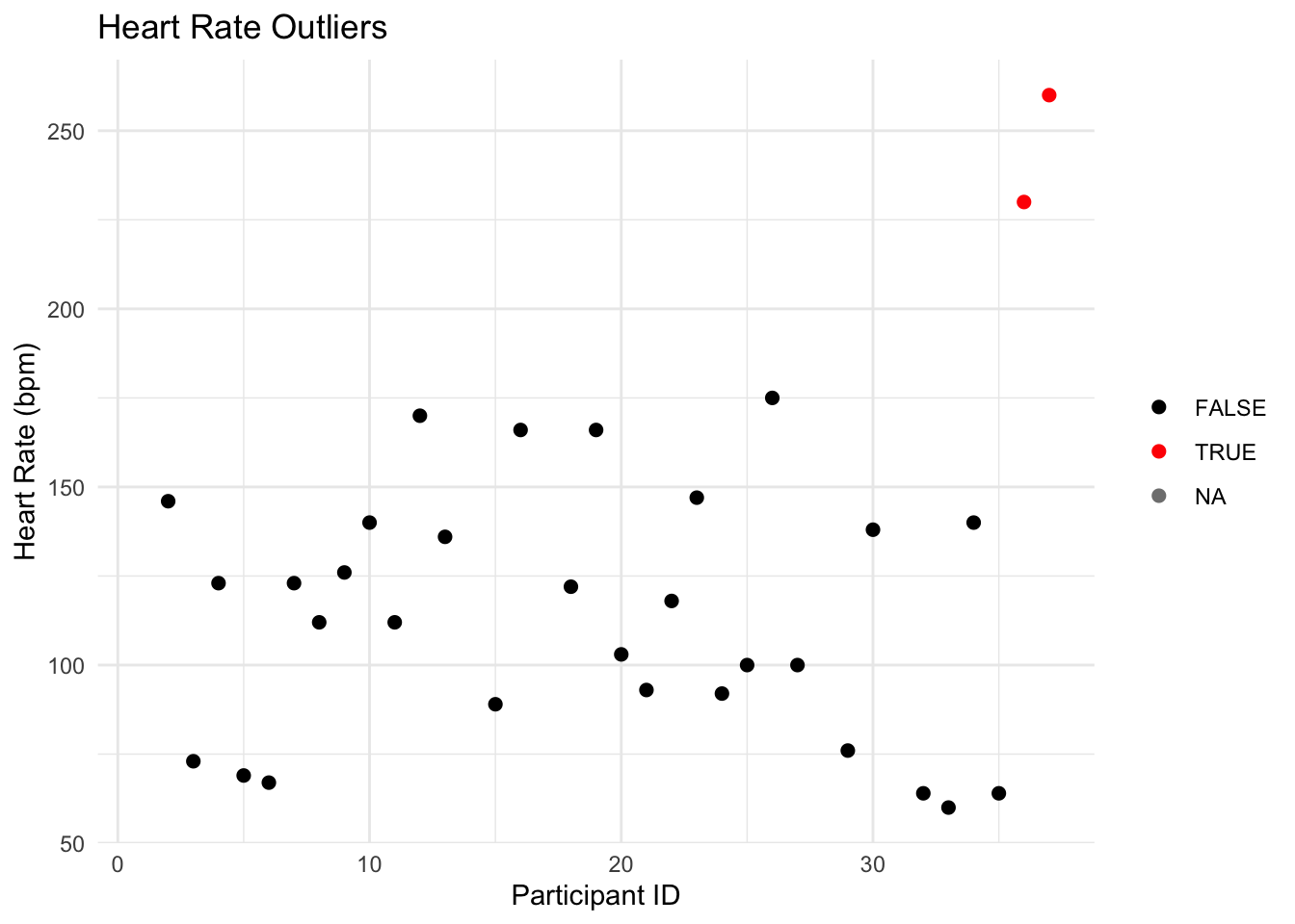
In this scatter plot, each point represents an individual measurement from the cycling_data dataset. We use color to differentiate outliers (in red) from the typical data points (in black), based on our previously defined criteria. This visualization not only shows the outliers but also situates them within the context of the entire dataset, offering a clear view of how they compare with the other data points.
By carefully identifying and visually examining outliers, we gain a fuller understanding of our dataset’s characteristics, enabling more informed decisions during data analysis and interpretation.
5.4 Handling Outliers in Your Dataset
Identifying outliers is a crucial step in data cleaning, but deciding how to handle them is equally important. Once outliers are detected — whether they are global, contextual, or collective — the next question is what to do with them. In exploratory data analysis (EDA), three primary strategies for handling outliers include deletion, reassignment, or retaining them in the dataset.
Deleting Outliers: This approach is suitable when there’s confidence that the outliers represent errors, such as data entry mistakes. Deletion should be considered carefully, especially for models or analyses where outlier removal could impact the results significantly. This method is generally less frequently employed.
Reassigning Outliers: For smaller datasets or in scenarios where the data will be used for modeling, deriving new values to replace outliers can be a viable option. Instead of removing outliers outright, their values can be adjusted to align with the general data distribution. This method helps preserve data integrity while mitigating the impact of outliers.
Leaving Outliers: Often, the best course of action might be to leave outliers in the dataset. This is particularly true for datasets intended for EDA or for models that are robust to the presence of outliers. Leaving outliers untouched is advisable when they provide valuable insights or when their removal could distort the analysis.
The decision to delete, reassign, or leave outliers in a dataset depends on the specific context and objectives of your analysis. Carefully consider the nature of your data and the potential implications of each approach to make the most informed decision.
By adopting a thoughtful strategy for handling outliers, you can ensure that your data analysis remains accurate and reflective of the underlying phenomena you’re investigating, enhancing the quality and reliability of your insights in sports and exercise science.
6 Conclusion and Reflection
In this lesson, we’ve navigated through the critical aspects of ensuring data integrity in sport and exercise science by focusing on handling missing data and outliers. With practical demonstrations using the cycling_data dataset, we’ve explored strategies for managing missingness through deletion and imputation, and identified and handled outliers to preserve the quality of our analysis. These techniques empower sports data analysts to maintain dataset integrity, enabling accurate and insightful interpretations that can enhance athletic performance and training strategies.
7 Knowledge Spot-Check
What is a common method to handle missing data in sports analytics?
A) Always delete missing values.
B) Replace missing values with the variable’s mean.
C) Ignore missing data during analysis.
D) Use machine learning to predict all missing values.
Expand to see the correct answer.
A) Always delete missing values.
B) Replace missing values with the variable’s mean.
C) Ignore missing data during analysis.
D) Use machine learning to predict all missing values.
Expand to see the correct answer.
The correct answer is B) Replace missing values with the variable’s mean.
Which type of outlier is an individual data point that significantly deviates from the rest?
A) Contextual outlier
B) Collective outlier
C) Global outlier
D) Standard outlier
Expand to see the correct answer.
A) Contextual outlier
B) Collective outlier
C) Global outlier
D) Standard outlier
Expand to see the correct answer.
The correct answer is C) Global outlier.
Why is it important to handle outliers in sports data analysis?
A) A) To ensure uniform data distribution.
B) To enhance the visual appeal of data plots.
C) To prevent them from skewing analysis results.
D) Outliers should never be handled; they represent true values.
Expand to see the correct answer.
A) A) To ensure uniform data distribution.
B) To enhance the visual appeal of data plots.
C) To prevent them from skewing analysis results.
D) Outliers should never be handled; they represent true values.
Expand to see the correct answer.
The correct answer is C) To prevent them from skewing analysis results.
Which R package is commonly used for Multiple Imputation by Chained Equations (MICE)
A) ggplot2
B) dplyr
C) mice
D) tidyr
Expand to see the correct answer.
A) ggplot2
B) dplyr
C) mice
D) tidyr
Expand to see the correct answer.
The correct answer is C) mice.
What is a practical approach for identifying outliers in a dataset?
A) Calculating the average speed of data entry.
B) Using a boxplot to visualize data distribution.
C) Counting the number of values above the mean.
D) Comparing datasets from different sports.
Expand to see the correct answer.
A) Calculating the average speed of data entry.
B) Using a boxplot to visualize data distribution.
C) Counting the number of values above the mean.
D) Comparing datasets from different sports.
Expand to see the correct answer.
The correct answer is B) Using a boxplot to visualize data distribution.