install.packages(c("tidyverse", "ggrepel", "ggsoccer", "RColorBrewer", "grid", "png", "gridExtra", "cowplot", "forcats"), repos="https://cloud.r-project.org/")Scatter Plots
Analyzing the Target: Scatter Plots Break Down the Matildas’ Shots at the FIFA Women’s World Cup 2023
Abstract
Visual insights drive decision-making, and scatter plots transform raw numbers into tangible patterns. This lesson highlights the invaluable utility of scatter plots within the expansive domain of Exploratory Data Analysis (EDA), with the FIFA Women’s World Cup 2023 data serving as our guiding dataset. Embark on a journey to understand the dynamics of scatter plots, a foundational EDA instrument, and unravel the nuances of the Matildas’ shooting strategies and tendencies. Designed for sports and exercise science practitioners, sports analysts, and anyone keen on mastering the art of sports data interpretation.
Keywords
Exploratory data analysis (EDA), exploratory data visualization (EDV), scatter plot, multidimensional scatter plot, tiled map of scatter plots, kernel density estimation, ggplot2, football, The Matildas, StatsBomb.
Lesson’s Level
The level of this lesson is categorized as BRONZE.
Lesson’s Main Idea
- Exploratory Data Analysis is about asking the right questions and using the appropriate visuals to glean insights.
- While numbers give us specifics, visualizations offer us perspective. Use visuals as a first step to understand your dataset.
- Scatter plots offer a visual representation of two variables and their relationships, enabling insights into patterns, trends, and potential anomalies.
- By harnessing scatter plots with additional layers, such as density estimations or aesthetics like shape and color, we can derive deeper insights and tell a more comprehensive story about the data.
Data used in this lesson is provided by ![]()
1 Learning Outcomes
By the end of this lesson, you will be proficient in:
Data Extraction and Preprocessing: Efficiently sourcing, processing, and refining datasets to ensure they are tailored for specific scatter plot visualizations.
Understanding Scatter Plots’ Role in EDA: Recognizing the unique capabilities of scatter plots in Exploratory Data Analysis (EDA) to visualize relationships and distributions of diverse variables.
Crafting Comprehensive Scatter Plots: Designing detailed scatter plot visualizations that effectively convey data points’ relationships, trends, and concentrations.
Implementing Advanced Scatter Plot Techniques: Leveraging advanced plotting methodologies and
ggplot2functionalities to enhance scatter plot representations with layered insights, annotations, and custom aesthetics.Analyzing and Drawing Conclusions from Scatter Plots: Cultivating the ability to extract meaningful insights from scatter plot data visualizations, underpinning data-driven decision-making across various domains.
2 Introduction: Exploring Connections Between Variables in Sports Science
2.1 Exploratory Data Analysis and Variable Relationships
In every discipline of sport and exercise science (SES), from biomechanics to physiology, variables do not operate in isolation. Their interactions, influences, and the outcomes they directly determine are the bedrock of these disciplines. For instance, consider the relationship between stride frequency and sprint speed in biomechanics, or the correlation between oxygen uptake and heart rate in physiology. Grasping how these variables correlate and interact is pivotal.
Exploratory Data Analysis (EDA) stands at the forefront of this understanding, serving as a tool to unravel these interactions. Once we comprehend the distribution of an individual variable, the progression in EDA involves delving into the relationships and impacts between variables. It prompts essential questions: How does a change in one variable affect another? Do they have a linear relationship, or is it more nuanced? Is there a discernible threshold where the impact shifts markedly?
The insights we glean from EDA, particularly when represented visually, empower sports and exercise science professionals. They can then anticipate patterns, fine-tune training regimes, adapt interventions, and ultimately elevate performance and well-being.
2.2 Unveiling Correlations and Trends Through Data Visualizations
In SES, effectively converting intricate interactions into discernible insights is often achieved through data visualizations, and scatter plots are a prime tool in this endeavor.
Consider the domain of physiology. A scatter plot can vividly depict the relationship between exertion and heart rate recovery, granting a snapshot of an athlete’s cardiovascular efficiency. In biomechanics, a plot can illuminate the correlation between force exerted and muscle fatigue. These visual representations unearth insights that might otherwise remain obscured in dense data.
Scatter plots are lauded for their directness. By juxtaposing two variables, they elucidate the nature of their interaction. This clarity is instrumental in formulating hypotheses and lays the foundation for in-depth statistical analyses. With a glance at a scatter plot, one can ascertain the type of relationship variables share and whether advanced modeling might be warranted. Consequently, scatter plots can catalyze predictive modeling and facilitate more intricate analyses.
In essence, scatter plots are an evolutionary step in EDA. While EDA deciphers the intricate dance of variables, scatter plots bring that dance to life, spotlighting patterns, relationships, and outliers, all invaluable assets in SES.
3 Scatter Plots
Scatter plots are foundational in data visualization for sport and exercise science, illuminating relationships between two numerical variables. When probing into the correlation between an athlete’s training duration and their subsequent performance or unveiling the ties between muscle exertion and recovery time, scatter plots shine as the instrument of choice.
3.1 What Are Scatter Plots?
A scatter plot is a graphical representation that displays individual data points on a two-dimensional plane. Each point corresponds to values from both the horizontal (X) and vertical (Y) variables. By visualizing these points, we can discern potential correlations, trends, or outliers between the two variables.
3.2 Types of Scatter Plots
Multidimensional Scatter Plot: An enhancement of the basic scatter plot, it introduces additional dimensions through attributes like the color, shape, or size of the points. In football, for instance, this might manifest as visualizing player positions on the pitch, while color-coding them based on metrics such as goals scored or distance run.
Tiled Map of Scatter Plots: Essentially, this is a matrix of scatter plots, each capturing a distinct subset of your data. Imagine a grid layout elucidating the evolution of player metrics like ball possession duration, passing accuracy, and shots on target over a series of matches or an entire season.
Scatter Plot with Kernel Density Estimation: By superimposing a density layer, it provides insights into areas of the plot with the highest concentration of data points. For a sport like football, this could illustrate zones on the field where most goals originate.
3.3 Strengths of Scatter Plots
Scatter plots excel in:
Identifying Correlations: Whether there’s a positive, negative, or no correlation, scatter plots offer clarity at a glance.
Spotting Outliers: They are adept at highlighting anomalies in your data, which can be crucial for sports analysis.
Diving Deep into Patterns: Scatter plots can reveal clusters or patterns, offering insights into, say, performance peaks or fatigue thresholds.
3.4 Harnessing ggplot2 for Scatter Plots
The ggplot2 library, a paramount tool in the R plotting ecosystem, will be our primary instrument in this lesson. Grounded in a layering principle, you initiate with a basic plot and progressively incorporate layers to refine both its utility and visual appeal. Each layer embeds more context or detail, making your plot progressively richer.
3.5 Functions for Scatter Plots in ggplot2
geom_point: The keystone function for scatter plots. Known for its adaptability, it enables detailed visual explorations, tailored to your dataset’s demands.
Attention to Scatter Plots
- Density Over Clutter: When dealing with dense datasets, consider the scatter plot with Kernel Density Estimation to avoid clutter.
- Scalability: As data volume grows, ensure clarity isn’t compromised by overcrowding.
- Axes Interpretation: Always ensure that the axes are correctly labeled and the scale is apt, ensuring accurate interpretation.
4 Case Study - Performance Insights from Scatter Plots at the FIFA Women’s World Cup 2023
Scatter plots, as powerful data visualization tools, transform seemingly complex numerical relationships into clear, interpretable patterns. With the assistance of these plots, intricate data can be demystified, enabling us to glean deeper insights. Turning our gaze towards the football statistics from the FIFA Women’s World Cup 2023, our objective becomes analyzing relationships in player performance metrics. We’ll particularly spotlight the Matildas - the Women’s Australian National Football Team. Through this exploration, we’ll highlight the essential role of scatter plots in elucidating connections and trends in sports statistics.
4.1 What to Expect
Scatter Plot - “Matilda’s Shooting Efficiency at FIFA Women’s World Cup 2023”: This visualization showcases the correlation between Non-Penalty Expected Goals per 90 Minutes (NPxG P90) and Shots per 90 Minutes. By using color to indicate average shot distance and shapes for goal scoring, we can explore: “Is the relationship between shots and expected goals linear?”, “How does average shot distance factor in?”, and “Which patterns can be seen in shooting efficiency?”
Tiled Scatter Plot - “Matildas’ Shot Maps at FIFA Women’s World Cup 2023”: In this plot, we’ll present the shot locations preferred by each Matildas player. This will help answer: “Where do players commonly shoot from?”, “How do different positions relate to the shot’s success?”, and “Which players have distinct shooting positions?”
Scatter Plot - “Penalty Shots Map”: This visualization provides insights into penalty shots during the tournament. We’ll seek to understand: “Where are penalties typically placed?” and “Which areas have the best success rates?”
With these visual tools, we’re ready to delve into the data and uncover the insights they offer.
4.2 Data Loading and Cleaning
In this lesson, we will utilize open-access data provided by StatsBomb - one of the world’s leading football analytics companies that provides high-quality football data. We will employ the StatsBombR package in R, which allows efficient access to the StatsBomb data.
To ensure a smooth execution of the code in this lesson, follow the steps below to install the necessary R libraries.
4.2.1 Installing Basic Libraries
Most of the libraries are readily available on CRAN and can be installed using the command install.packages("NameOfPackage"), if they are not already installed on your computer:
4.2.2 Installing From GitHub
Some packages, such as StatsBombR, are not available on CRAN and need to be installed from GitHub. This can be achieved using the devtools package. If you have not already, please install devtools:
install.packages("devtools", repos="https://cloud.r-project.org/")In order to install packages from GitHub, ensure Git is also set up on your machine1. If it is not installed, download and install Git. This will allow devtools to clone and install packages from GitHub directly.
Now, the StatsBombR package can be installed using the following command:
devtools::install_github("statsbomb/StatsBombR")After you have installed all the required packages, you can load them into your current R session as follows:
rm(list = ls()) # clean the workspace

# Load required libraries
library(StatsBombR)    # For accessing and handling StatsBomb football data
library(tidyverse)     # For data manipulation and visualization
library(ggrepel)       # To avoid label overlap in plots
library(ggsoccer)      # For plotting soccer pitches
library(RColorBrewer)  # For colorblind-friendly palettes
library(grid)          # For lower-level graphics functions
library(png)           # To read and write PNG images
library(gridExtra)     # For arranging multiple grid-based plots
library(cowplot)       # For enhancing and customizing ggplot figures
library(forcats)       # For categorical variable (factor) manipulation
4.2.3 Pulling and Organizing StatsBomb Data
Explore the Code
This lesson features annotated code sections, with comments elucidating the intent and operation of every code snippet. Nonetheless, to genuinely grasp the influence of a particular plot customization function, it is advisable to momentarily comment out that specific code line and see the consequent modifications in the graphic. For RStudio users on macOS, the keyboard shortcut to comment out a line or multiple lines of code is .
The initial step involves retrieving and loading the StatsBomb dataset, followed by the extraction of relevant data for this lesson. The code provided below accomplishes this task.
# ---- Load and Tidy Up StatsBomb data ----

#* Pull and load free StatsBomb data ----

# Measure the time it takes to execute the code within the system.time brackets (for performance)
system.time({
  # Fetch list of all available competitions
  all_comps <- FreeCompetitions()

  # Filter to get only the 2023 FIFA Women's World Cup data (Competition ID 72, Season ID 107)
  Comp <- all_comps %>%
    filter(competition_id == 72 & season_id == 107)

  # Fetch all matches of the selected competition
  Matches <- FreeMatches(Comp)

  # Download all match events and parallelize to speed up the process
  StatsBombData <- free_allevents(MatchesDF = Matches, Parallel = T)

  # Clean the data
  StatsBombData = allclean(StatsBombData)
})

# Show the column names of the final StatsBombData dataframe
names(StatsBombData)
After loading the data and briefly examining it to acquaint ourselves with the structure of the StatsBombData dataframe, we can proceed to refine the team names.
#* Tidy up the teams' names ----

# Create a dataframe containing unique names of all teams at FWWC23
WWC_teams <- data.frame(team_name = unique(StatsBombData$team.name))

# Remove the " Women's" part from team names for simplicity
StatsBombData$team.name <- gsub(" Women's", "", StatsBombData$team.name)

# Rename and simplify team names in the 'Matches' dataframe
Matches <- Matches %>%
  rename(
    home_team = home_team.home_team_name,
    away_team = away_team.away_team_name
  ) %>%
  mutate(
    home_team = gsub(" Women's", "", home_team),
    away_team = gsub(" Women's", "", away_team)
  )
Having set the stage, we are now poised to delve into data analysis and construct scatter plot visualizations for our chosen metrics. We will kick off with the “Matildas’ Shooting Efficiency” scatter plot.
4.3 Multidimensional Scatter Plot
In this section, we craft a scatter plot contrasting shots per 90 minutes (shots_p90) against non-penalty expected goals per 90 minutes metric (npxg_p90). This visualization sheds light on a player’s shooting frequency relative to the quality of those shots, offering insights into overall shooting efficiency.
4.3.1 Data Filtering
The code below parses through the StatsBombData dataframe, selecting specific columns pertinent to our scatter plot analysis. It focuses on the shots taken by the Matildas, excluding penalty shots. The shot outcomes are categorized into five distinct types: Goal, Off T (Off Target), Saved, Saved to Post, and Post.
# Extract relevant shot data for Matildas from StatsBombData
shots_Matildas <- StatsBombData%>%
  select(player.name, player.id, team.name, team.id, type.name, shot.type.name, shot.outcome.name, shot.statsbomb_xg, location.x, location.y, DistToGoal)%>%
  filter(team.name == "Australia")%>%
  filter(type.name == "Shot" & (shot.type.name != "Penalty"|is.na(shot.type.name)))%>%
  filter(shot.outcome.name %in% c("Goal", "Off T", "Saved", "Saved to Post", "Post"))
Having refined our dataset, we can now efficiently analyze the Matildas’ shooting performance.
4.3.2 Extracting Players’ Last Names
To streamline the dataframe with the Matildas’ shot data, we will add a column capturing players’ last names. This aids in annotating points on the scatter plot with player names. Using the extract_last_name function, we also cater to names that include “van”. Finally, we reposition the ‘last_name’ column to follow ‘player.name’.
# Function to extract the last name from a full name string
extract_last_name <- function(full_name) {
  name_parts <- strsplit(full_name, " ")[[1]]

  # Check if the name contains "van"
  if ("van" %in% name_parts) {
    # Concatenate "van" with the last name
    return(paste("van", tail(name_parts, 1), collapse = " "))
  } else {
    # Just return the last name
    return(tail(name_parts, 1))
  }
}

# Add a new column for players' last names
shots_Matildas$last_name <- sapply(shots_Matildas$player.name, extract_last_name)

# Reorder the columns to have last_name after player.name
shots_Matildas <- shots_Matildas %>%
  select(player.name, last_name, everything())
4.3.3 Computing Stats Per Player
In this step, we structure our data around individual players. For each player, we count the number of non-penalty shots taken, sum up the non-penalty expected goals metric (npxg), and calculate the average distance to the goal (avg_dist) for their shots. Additionally, the code determines whether a player has scored a goal (scored_goal), considering only non-penalty shots.
# Calculate stats for each player
# Group by player and compute the following metrics: the number of shots they have taken, total NPxG, average distance to goal, and whether a player scored a goal
shots_Matildas_stats <- shots_Matildas%>%
  group_by(player.name, player.id, last_name)%>%
  summarise(shots=sum(type.name=="Shot", na.rm=TRUE),
            npxg=sum(shot.statsbomb_xg),
            avg_dist = mean(DistToGoal, na.rm = TRUE),
            scored_goal = any(shot.outcome.name == "Goal"),
            .groups = "drop")
Note
Using .groups = 'drop' effectively ungroups the data, making the dataframe easier to manage and the code more explicit.
4.3.4 Normalizing Metrics to 90 Minutes of Play
In this section, we first determine the total minutes played by each Matilda by leveraging the overall minutes played by all players. With the accumulated minutes, we then compute metrics normalized to a 90-minute game duration, notably shots_p90 and npxg_p90. Furthermore, to facilitate clearer visual representation, we categorize average shot distances into distinct bins (avg_dist_binned). This categorization aids in providing a structured overview of the players’ shooting distances.
# Get the total minutes played by each player
all_players_minutes = get.minutesplayed(StatsBombData)

# Extract Australia's team ID
Australia_team_id <- unique(shots_Matildas$team.id)

# Sum up the total minutes played by each Matilda
Matildas_minutes <- all_players_minutes %>%
  filter(team.id == Australia_team_id) %>%
  group_by(player.id) %>%  # Group data by player.id
  summarise(total_minutes_played = round(sum(MinutesPlayed), digits = 2), # Sum up total minutes played
            .groups = "drop")

# Join the minutes data with the shot stats data
shots_Matildas_stats <- shots_Matildas_stats%>%
  left_join(Matildas_minutes, by = "player.id")

# Normalize shots and NPxG per 90 minutes of play
shots_Matildas_stats <- shots_Matildas_stats%>%
  mutate(nineties = round(total_minutes_played/90, digits=2))

shots_Matildas_stats <- shots_Matildas_stats%>%
  mutate(shots_p90 = shots/nineties,
         npxg_p90 = npxg/nineties)

# Bin the average distance
shots_Matildas_stats <- shots_Matildas_stats %>%
  mutate(avg_dist_binned = cut(avg_dist, breaks = seq(0, max(avg_dist) + 10, by = 10)))

# Convert to factors for easier plotting
shots_Matildas_stats$avg_dist_binned <- as.factor(shots_Matildas_stats$avg_dist_binned)
shots_Matildas_stats$scored_goal <- as.factor(shots_Matildas_stats$scored_goal)
4.3.5 Creating the Multidimensional Scatter Plot
Now we are ready to visualize the Matildas’ shooting efficiency with a scatter plot. The x-axis depicts shots_p90, indicating the frequency of shots taken per 90 minutes of play. On the y-axis, we have npxg_p90, showcasing the non-penalty expected goals metric also normalized to 90 minutes. Each point’s fill color corresponds to the average shot distance (avg_dist_binned), while its shape indicates whether the player has scored. The annotations on the scatter plot help identify each player by their last name.
Scatter Plot Point Shape Values
To explore different point shape values, first install the ggpubr package using install.packages("ggpubr"). Then, call show_point_shapes().
# Create the scatter plot
shot_effic_viz <- ggplot(data=shots_Matildas_stats,
       aes(x = shots_p90,
           y = npxg_p90)) +
  geom_point(aes(fill = avg_dist_binned,
                 shape = scored_goal),
             size = 6,
             stroke = 0.6,
             colour = "black",
             alpha = 0.8) +
  geom_text_repel(data = shots_Matildas_stats,
                  aes(x = shots_p90,
                      y = npxg_p90,
                      label = last_name),
                  size = 5.5, #4.5
                  box.padding = 0.5,
                  point.padding = 0.5) +
  xlim(0, 4) +
  ylim(0, 0.3) +
  scale_shape_manual(values = c("FALSE" = 21, "TRUE" = 24), name ="",
                     labels = c("Not Scored", "Scored")) +
  scale_fill_manual(values = c("#1abc9c", "#e74c3c", "#9b59b6", "#f1c40f"), name = "Av. Shot Dist. [m]",
                    labels = c("0-10", "10-20", "20-30", "30-40")) +
  guides(fill = guide_legend(override.aes = list(shape = 22)),
         shape = guide_legend(override.aes = list(fill = "black"))) +
  theme(
    # Set background color to white
    panel.background = element_rect(fill = "white"),
    # Set the color and the width of the grid lines
    panel.grid.major.y = element_line(color = "#A8BAC480", size = 0.3),
    # Set the color and the width of the grid lines
    panel.grid.major.x = element_line(color = "#A8BAC480", size = 0.3),
    # Remove tick marks by setting their length to 0
    axis.ticks.length = unit(0, "mm"),
    # Customize the title for both axes
    axis.title = element_text(family = "sans", size = 16, color = "black"),
    # Labels for the horizontal axis
    axis.text.x = element_text(family = "sans", size = 16, color = "black"),
    # Labels for the vertical axis
    axis.text.y = element_text(family = "sans", size = 16, color = "black"),
    legend.text = element_text(family = "sans", size = 16, color = "black"), #12
    legend.position = "right",
    legend.key = element_blank(),
    legend.title = element_text(family = "sans", size = 16, face = "bold", color = "black") #14
  ) +
  labs(title = "Matildas' Shooting Efficiency at FIFA Women's World Cup 2023",
       subtitle = "Non-Penalty Expected Goals per 90 Minutes (NPxG P90) vs Shots per 90 Minutes\nColored by Average Shot Distance and Shaped by Goal Scoring",
       x = "Shots P90",
       y = "NPxG P90") +
  theme(
    plot.title = element_text(
      family = "sans",
      face = "bold",
      size = 16,
      color = "black"
    ),
    plot.subtitle = element_text(
      family = "sans",
      size = 16,
      color = "black"
    )
  )
4.3.6 Adding the StatsBomb Logo
The StatsBomb logo is inserted into the bottom right corner of the plot.
Warning
To ensure the code below runs smoothly, download the required StatsBomb logo from here and save it in the same directory as your R script file. In the script, you can then use a relative path to load the image (e.g., ‘img_path’ for a filename like ‘SB_logo.png’). Remember, for the relative path to work, the working directory should be set to where the script is. In R, use getwd() to check the current directory and setwd("/path/to/directory") to set it.
# Specify the path to the StatsBomb logo image
img_path <- "SB_logo.png"

# Add the StatsBomb logo to the existing plot
shot_effic_viz_sb <- ggdraw(shot_effic_viz) +
  draw_image(img_path, x = 0.87, y = 0, width = 0.12, height = 0.06)

# Add a label to indicate the data source
shot_effic_viz_sb <- ggdraw(shot_effic_viz_sb) +
  draw_label("Data:", x = 0.84, y = 0.03, size = 16)

# Display the finalized plot
print(shot_effic_viz_sb)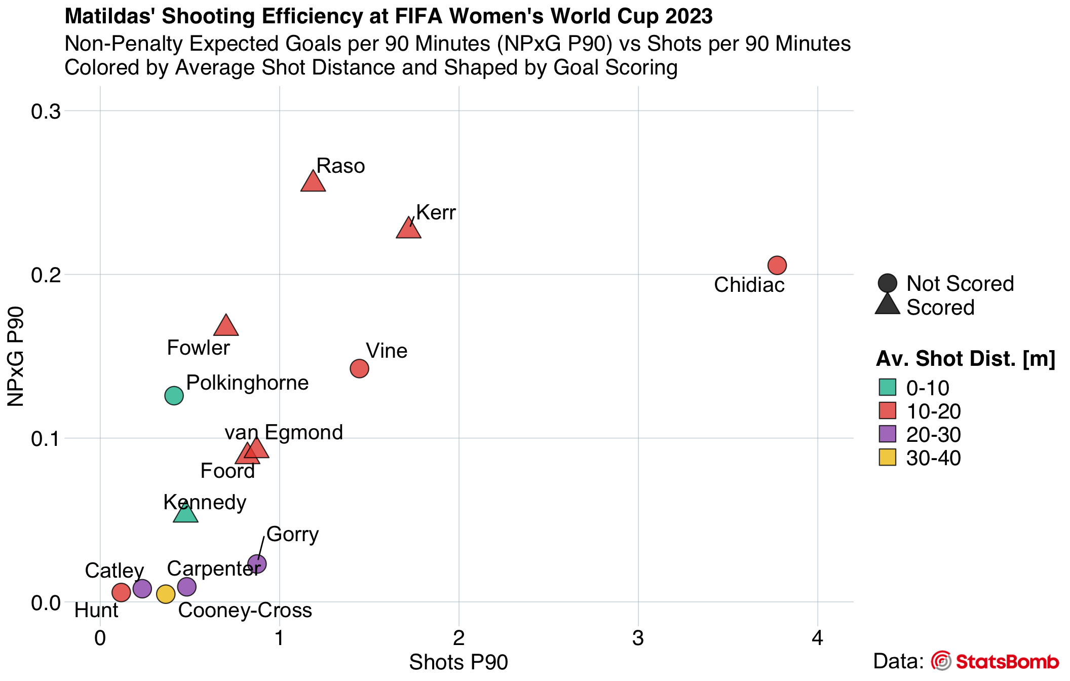
#* Save the visualization to png ----

# ggsave("Matildas_Shooting_Efficiency.png", plot = shot_effic_viz_sb, width = 10, height = 8, dpi = 300)
4.4 Tiled Map of Scatter Plots
In this section, we craft a tiled map of scatter plots showcasing the preferred shot locations of each Matildas player during the FIFA Women’s World Cup 2023. This visualization offers insights into common shooting positions, their correlation with shot success, and the unique shooting tendencies of individual players.
4.4.1 Refining Data
To differentiate between successful shots and misses, we introduce a new column, shot_outcome, that labels each shot as either “Goal” or “No Goal”, determined by the shot.outcome.name value.
# Add a new column to categorize each shot as either a "Goal" or "No Goal"
shots_Matildas <- shots_Matildas %>%
  mutate(shot_outcome = ifelse(shot.outcome.name == "Goal", "Goal", "No Goal"))
4.4.2 Creating the Tiled Map of Scatter Plots
Football Pitch Visualization
To visualize a football pitch, we employ the ggsoccer library. While this provides a convenient method, one can also craft a pitch using the annotate() function from ggplot2. By varying its first argument, shapes such as rect, segment, point, and path can be utilized to manually construct the pitch.
# Initialize an empty ggplot object
shot_map_viz <- ggplot() +
  # Draw the soccer pitch
  annotate_pitch(dimensions = pitch_statsbomb,
                 colour = "white",
                 fill = "springgreen4",
                 limits = FALSE) +
  theme_pitch() +
  # Set background color
  theme(panel.background = element_rect(fill = "springgreen4")) +
  # Flip x and y axes to orient the pitch vertically
  coord_flip(xlim = c(60, 120)) +
  # Reverse y-axis
  scale_y_reverse() +
  # Plot each Matildas' shot
  geom_point(data = shots_Matildas,
             aes(x = location.x,
                 y = 80 - location.y,
                 fill = shot_outcome,
                 size = shot.statsbomb_xg),
             shape = 21, # Circle shape
             stroke = 0.3, # Circle border thickness
             colour = "black") + # Circle border color
  # Manually set the colors for shot outcomes
  scale_fill_manual(values = c("Goal" = "#e74c3c", "No Goal" = "#f1c40f"),
                      name = "Shot Outcome",
                      labels = c("Goal", "No Goal")) +
  guides(size = guide_legend(override.aes = list(fill = "#f1c40f")),
         fill = guide_legend(override.aes = list(size = 3))) +
  # Create panels for each player's shot map
  facet_wrap(~last_name) +
  # Add statistics for shots per 90 minutes, NPxG per 90 minutes, and average shot distance
  geom_text(data = shots_Matildas_stats,
            aes(x=80,
                y=80-15,
                label = paste("Shots P90:", round(shots_p90, digits=3))),
            size = 2.7) + #2.2
  geom_text(data = shots_Matildas_stats,
            aes(x=74,
                y=80-15,
                label = paste("NPxG P90:", round(npxg_p90, digits=3))),
            size = 2.7) +
  geom_text(data = shots_Matildas_stats,
            aes(x=68,
                y=80-15,
                label = paste("Avg. Dist.:", round(avg_dist, digits=3))),
            size = 2.7) +
  theme(
    # Set background color to white
    panel.background = element_rect(fill = "white"),
    # Set the color and the width of the grid lines
    panel.grid.major.y = element_blank(),
    # Set the color and the width of the grid lines
    panel.grid.major.x = element_blank(),
    # Remove tick marks by setting their length to 0
    axis.ticks.length = unit(0, "mm"),
    # Customize the title for both axes
    axis.title = element_blank(),
    # Labels for the horizontal axis
    axis.text.x = element_blank(),
    # Labels for the vertical axis
    axis.text.y = element_blank(),
    legend.text = element_text(family = "sans", size = 16, color = "black"), #12
    legend.position = "top",
    legend.key = element_blank(),
    legend.title = element_text(family = "sans", size = 16, face = "bold", color = "black"), # 14
    strip.text = element_text(hjust = 0.5, size = 16, face = "bold"), #12
    strip.background = element_blank()
  ) +
  labs(title = "Matildas' Shot Maps at FIFA Women's World Cup 2023",
       subtitle = "Only Non-Penalty Shots That Reached the Goal",
       size = "Non-Penalty xG") +
  theme(
    plot.title = element_text(
      family = "sans",
      face = "bold",
      size = 16,
      color = "black",
      hjust = 0.5
    ),
    plot.subtitle = element_text(
      family = "sans",
      size = 16,
      color = "black",
      hjust = 0.5
    )
  )
4.4.3 Adding the StatsBomb Logo
The StatsBomb logo is inserted into the bottom right corner of the plot.
Warning
To ensure the code below runs smoothly, download the required StatsBomb logo from here and save it in the same directory as your R script file. In the script, you can then use a relative path to load the image (e.g., ‘img_path’ for a filename like ‘SB_logo.png’). Remember, for the relative path to work, the working directory should be set to where the script is. In R, use getwd() to check the current directory and setwd("/path/to/directory") to set it.
# Insert the StatsBomb logo ----
img_path <- "SB_logo.png"

shot_map_viz_sb <- ggdraw(shot_map_viz) +
  draw_image(img_path, x = 0.7, y = 0, width = 0.13, height = 0.065)

# Add a label indicating the data source
shot_map_viz_sb <- ggdraw(shot_map_viz_sb) +
  draw_label("Data:", x = 0.67, y = 0.033, size = 16)

# Display the final plot
print(shot_map_viz_sb)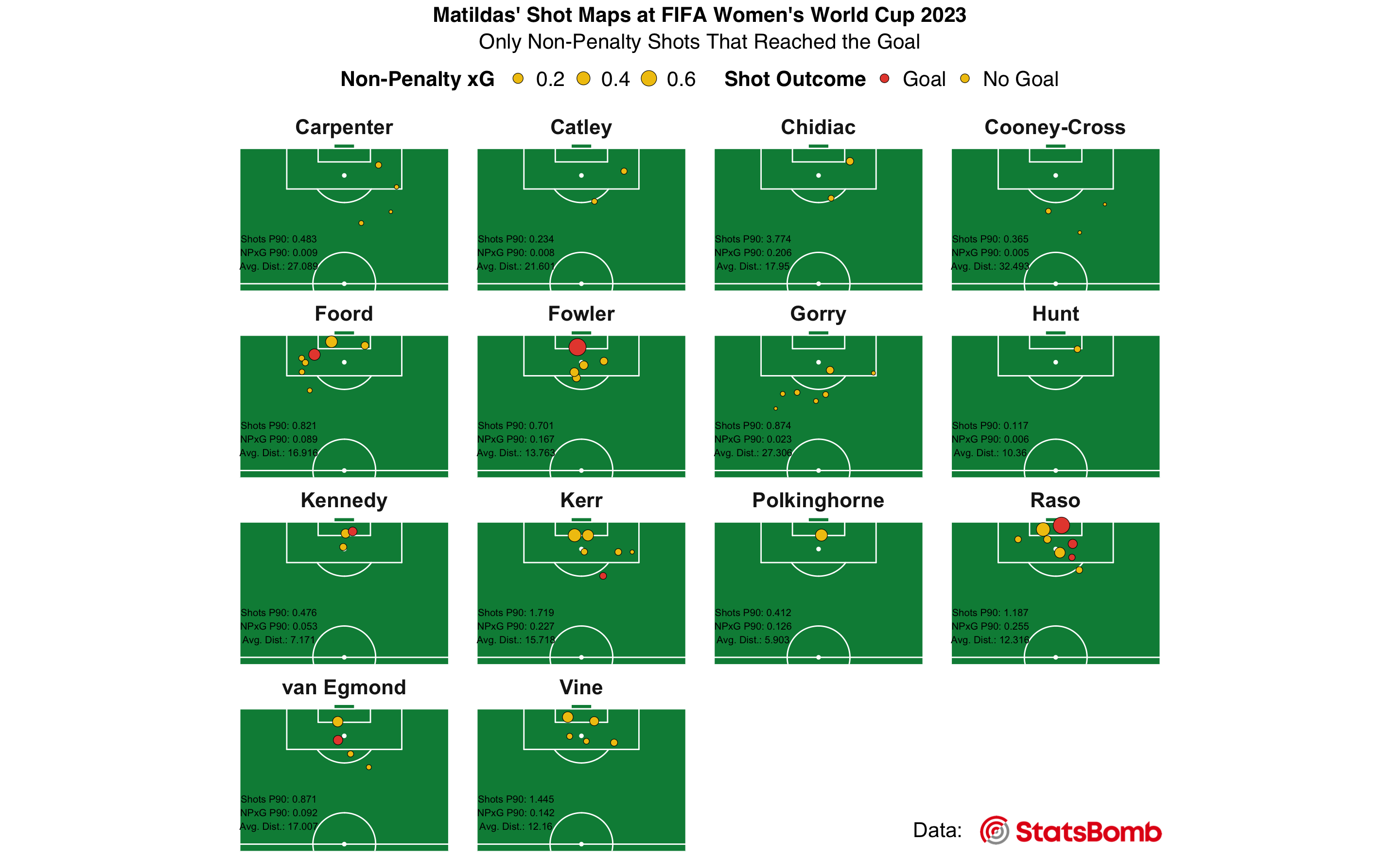
#* Save the visualization to png ----

# ggsave("Matildas_Shot_Maps.png", plot = shot_map_viz_sb, width = 10, height = 8, dpi = 300)
4.5 Scatter Plot with Kernel Density Estimation
In this section, we delve into a scatter plot enhanced with kernel density estimation, highlighting zones of the goal where penalty shots were most frequently placed during the FIFA Women’s World Cup 2023. This includes both in-game penalties and penalty shootouts. By identifying where successful (scored) penalties tend to land within the goal frame, we offer a clearer picture of player preferences and tendencies. Additional annotations and layers, like text labels, are incorporated for context and clarity.
4.5.1 Data Filtering - All Penalties
First, we extract data on all penalties from the FIFA Women’s World Cup 2023, including in-game shots and shootouts, by refining the StatsBombData dataset to retain only pertinent penalty shot details.
# Check each column to see if it contains the word "Penalty"
penalty_columns <- sapply(StatsBombData, function(x) any(x == "Penalty", na.rm=TRUE))
# Keep the names of columns where "Penalty" is found
penalty_columns <- names(penalty_columns[penalty_columns == TRUE])

# Display columns containing "Penalty"
penalty_columns
[1] "shot.type.name"# Select specific columns to keep for the penalty analysis
selected_columns <- c("match_id", "player.name", "team.name", penalty_columns,
"shot.outcome.name", "shot.end_location.x",
"shot.end_location.y", "shot.end_location.z", "period")
# Filter only the rows where shot type is "Penalty"
all_penalties <- StatsBombData%>%
select(all_of(selected_columns))%>%
filter(shot.type.name == "Penalty")
# Rename columns to be more readable
all_penalties <- all_penalties %>%
rename(
penalty_taker = player.name,
penalty_taker_team = team.name,
match_phase = period
)4.5.2 Feature Engineering
Here, we categorize the penalties based on what match phase they were taken in (in-game or penalty shootout) and what the outcome was.
# Add a new column 'match_phase' to indicate when the penalty was taken (In-game or Shootout)
all_penalties <- all_penalties%>%
  mutate(
    match_phase = case_when(
      match_phase %in% 1:4 ~ "In-Game",
      match_phase == 5 ~ "Penalty Shootout",
      TRUE ~ as.character(match_phase)
    )
  )

# Join 'Matches' data to get home and away teams
all_penalties <- all_penalties%>%
  left_join(Matches %>% select(match_id, home_team, away_team), by = "match_id")

# Create a column 'shot_outcome' to simplify shot outcome into "Goal" or "Missed"
all_penalties <- all_penalties %>%
  mutate(shot_outcome = ifelse(shot.outcome.name == "Goal", "Goal", "Missed"))

# Reorder the columns
all_penalties <- all_penalties %>%
  select(match_id, home_team, away_team,
         penalty_taker, penalty_taker_team,
         shot.type.name, match_phase,
         shot.outcome.name, shot_outcome, shot.end_location.x,
         shot.end_location.y, shot.end_location.z)
4.5.3 Building the Scatter Plot with Kernel Density Estimation
4.5.3.1 Initializing the Plot
Set up the initial ggplot object.
# Filter successful and unsuccessful penalties
scored_penalties <- all_penalties %>% filter(shot.outcome.name == "Goal")
missed_penalties <- all_penalties %>% filter(shot.outcome.name != "Goal")

# Define dimensions for the goal and plot area
floor = 0
x_left = 36
x_right = 44
y_crossbar = 2.8

canvas_left = 34.9
canvas_right = 45.2
canvas_top = 6.5
canvas_bottom = -0.9

# Initialize ggplot
pen_viz <- ggplot() +
  xlim(canvas_left, canvas_right) + ylim(canvas_bottom, canvas_top) +
  coord_fixed(ratio = 0.9) +
  labs(title="Penalty Shots Map",
       subtitle = "All penalty shots (both in-game and shootouts) at FIFA Women's World Cup 2023") +
  # Customize plot appearance
  theme(plot.title = element_text(color="black", size=16, face="bold", hjust = 0.5),
        plot.subtitle = element_text(color="black", size=16, hjust = 0.5),
        panel.grid.major = element_blank(),
        panel.grid.minor = element_blank(),
        axis.title.x = element_blank(),
        axis.title.y = element_blank(),
        axis.ticks = element_blank(),
        axis.text.x = element_blank(),
        axis.text.y = element_blank(),
        panel.background = element_rect(fill = "white"),
        plot.background = element_rect(fill = "white"))

# Define line thickness for the goal frame
goal_frame_thick <- 4
4.5.3.2 Creating a Density Plot
Overlay a density plot to visualize the distribution of successful penalty shots within the goal frame.
Warning
A ball icon required for the code below can be downloaded here. After downloading, ensure you specify your own path to the ball icon in the code. If you’ve saved the ball icon in the same directory as your R script file, you can use a relative path. Alternatively, if you prefer not to use any images for your scatter plot points, simply omit the portion of the code that loads and applies the ball icon.
# Add density plot for successful penalties
pen_viz <- pen_viz +
  stat_density_2d(data=scored_penalties, geom = "polygon",
                  aes(x=shot.end_location.y, y=shot.end_location.z, fill = after_stat(level)),
                  alpha = 0.2, bins = 500) +
  scale_fill_gradientn(name = "Penalty Scoring Density",
                       colours=rev(brewer.pal(7, "RdYlBu"))) + #Spectral
  theme(legend.position = c(0.58, 0.06),
        legend.direction = "horizontal",
        legend.title = element_text(size = 14, color = "black"),
        legend.key.size = unit(0.7, "cm"),
        legend.text = element_blank(),
        legend.key = element_blank(),
        legend.background = element_rect(fill = "white")) +
  guides(fill = guide_colourbar(title.position="top", title.hjust = 0.5))

# Clip density plot to the goal frame dimensions
pen_viz <- pen_viz +
  geom_rect(aes(xmin = canvas_left, xmax = x_left, ymin = canvas_bottom, ymax = canvas_top),
            fill = "white") +
  geom_rect(aes(xmin = x_right, xmax = canvas_right, ymin = canvas_bottom, ymax = canvas_top),
            fill = "white") +
  geom_rect(aes(xmin = x_left, xmax = x_right, ymin = y_crossbar, ymax = canvas_top),
            fill = "white") +
  geom_rect(aes(xmin = x_left, xmax = x_right, ymin = canvas_bottom, ymax = floor),
            fill = "white")

# Define data for drawing the goal frame
goal_frame_data <- data.frame(
  x = c(x_left, x_left, x_right, x_right),
  y = c(floor, y_crossbar, y_crossbar, floor)
)

# Draw the goal frame
pen_viz <- pen_viz +
  geom_path(data=goal_frame_data, aes(x=x, y=y),
            color="black", size=goal_frame_thick)


# Load a ball symbol png file
img <- readPNG("ball_symbol.png")

# Create a raster graphical object
ball <- rasterGrob(img, interpolate=TRUE)

ball_size = 0.15

# Add the red crosses for the 'Missed' penalties
pen_viz <- pen_viz + geom_point(data = missed_penalties,
                                aes(x=shot.end_location.y, y=shot.end_location.z),
                                shape = 4, color = '#e74c3c', size = 3, stroke = 2)

# Loop through each row in the dataframe with 'Goal' penalties
for(i in 1:nrow(scored_penalties)) {

  # Extract the current shot's coordinates
  x <- scored_penalties$shot.end_location.y[i]
  y <- scored_penalties$shot.end_location.z[i]

  # Annotate with the ball image
  pen_viz <- pen_viz + annotation_custom(ball,
                                         xmin = x - ball_size, xmax = x + ball_size,
                                         ymin = y - ball_size, ymax = y + ball_size)
}
4.5.3.3 Adding Annotations
Here, we annotate two particular penalty shots from the Australia v France FWWC23 quarterfinal. One penalty is by Mackenzie Arnold and the other one is by Cortnee Vine - two memorable penalty shots for all Aussies!
# Coordinates for both penalties
symbol_x_scored = 42.2
symbol_y_scored = 0.2

symbol_x_missed = 44.0
symbol_y_missed = 1.6


# Create a data frame containing the points to be annotated
annotate_data <- data.frame(
  x = c(symbol_x_scored, symbol_x_missed),
  y = c(symbol_y_scored, symbol_y_missed),
  label = c("C. Vine", "M. Arnold")
)

pen_viz <- pen_viz +
  geom_text_repel(data = annotate_data,
                   aes(x = x, y = y, label = label),
                   box.padding = 0.5,  # Space around each label
                   point.padding = 0.5,  # Space around each point
                   segment.color = "#9b59b6",
                   segment.size = 1.5,
                   nudge_x = 0.9,  # Horizontal adjustment
                   nudge_y = -0.4,  # Vertical adjustment
                   direction = "both",  # ('x' or 'y'): Direction in which to move labels
                   arrow = arrow(type = "closed", length = unit(2.1, "mm")),
                   size = 6,
                   color = "#9b59b6") # Text size and color
4.5.4 Adding the StatsBomb Logo
Add the StatsBomb logo, a legend for scored and missed penalties, and save the plot.
Warning
To ensure the code below runs smoothly, download the required StatsBomb logo from here and save it in the same directory as your R script file. In the script, you can then use a relative path to load the image (e.g., ‘img_path’ for a filename like ‘SB_logo.png’). Remember, for the relative path to work, the working directory should be set to where the script is. In R, use getwd() to check the current directory and setwd("/path/to/directory") to set it.
# Insert the Statsbomb logo and the legend ----
img_path_SB_logo <- "SB_logo.png"
img_path_ball <- "ball_symbol.png"

pen_viz_sb <- ggdraw(pen_viz) +
  draw_image(img_path_SB_logo, x = 0.735, y = 0.06, width = 0.13, height = 0.065)
pen_viz_sb <- ggdraw(pen_viz_sb) +
  draw_label("Data:", x = 0.71, y = 0.09, size = 16)

pen_viz_sb <- ggdraw(pen_viz_sb) +
  draw_image(img_path_ball, x = 0.27, y = 0.07, width = 0.07, height = 0.035)
pen_viz_sb <- ggdraw(pen_viz_sb) +
  draw_label("Scored", x = 0.25, y = 0.09, size = 16)


x_center <- 0.43  # x-coordinate of the center of the cross
y_center <- 0.09  # y-coordinate of the center of the cross
length <- 0.02    # length of each arm of the cross from the center
x1 <- x_center - length / sqrt(2)
y1 <- y_center - length / sqrt(2)
x2 <- x_center + length / sqrt(2)
y2 <- y_center + length / sqrt(2)

pen_viz_sb <- pen_viz_sb +
  geom_point() +
  annotate("segment", x = x1, xend = x2, y = y1, yend = y2, color = "#e74c3c", size = 1) +
  annotate("segment", x = x1, xend = x2, y = y2, yend = y1, color = "#e74c3c", size = 1)


pen_viz_sb <- ggdraw(pen_viz_sb) +
  draw_label("Missed", x = 0.38, y = 0.09, size = 16)

# Show the final visualization
print(pen_viz_sb)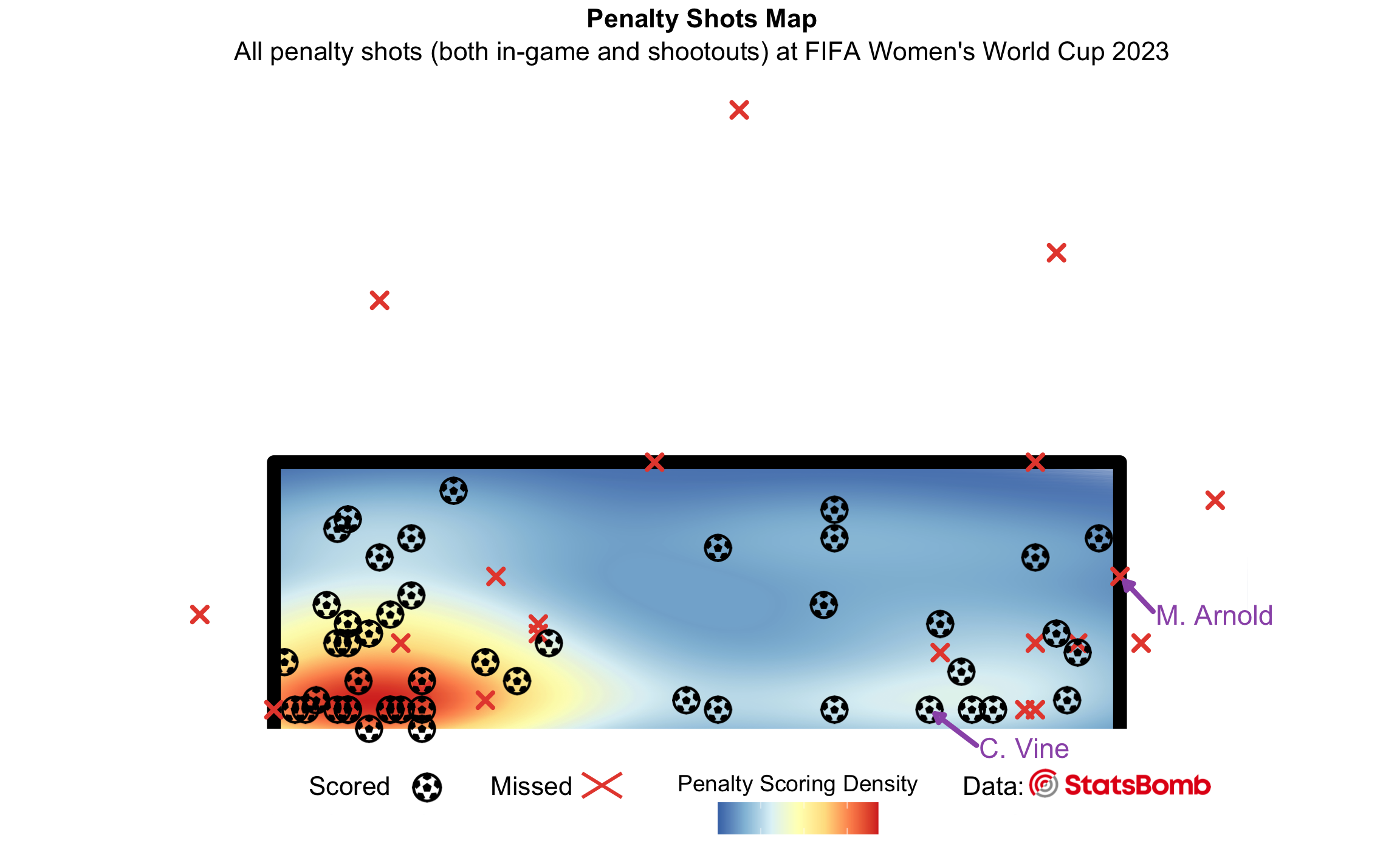
#* Save the visualization to png ----
# ggsave("Penalty_Shots_Map.png", plot = pen_viz_sb, width = 10, height = 8, dpi = 300)
Challenge for the Learner
Strengthen your understanding of scatter plots and the FIFA Women’s World Cup 2023 data by:
- Creating a scatter plot comparing shot accuracy (shots on target vs. total shots) for the top 10 players with the most shots.
- Visualizing a scatter plot with kernel density estimation for shots taken from outside the penalty box across all teams, highlighting zones with the highest goal conversion rates.
5 Conclusion and Reflection
Scatter plots, as we have seen, are powerful tools in sports data visualization. They excel in revealing relationships between variables, offering a depth of insight that surpasses basic statistical summaries. In this lesson, we delved into how these plots can shed light on the relationships between variables, such as the connection between shooting efficiency and the number of shots taken per game.
But their utility isn’t confined to just performance metrics. Their foundational principle—visualizing relationships between variables—can be applied across various domains. For instance, in physiology, one might use scatter plots to study the link between heart rate variability and exercise intensity. Similarly, biomechanists could use them to investigate the connection between joint angles and performance.
As we used the Matildas’ performance data from the FIFA Women’s World Cup 2023 as our primary example, it is essential to remember that the broader EDA techniques and principles remain consistent across different sports science disciplines. It’s about systematically identifying patterns, asking the right questions, and selecting the appropriate visualization tools to derive insights.
Moving forward, understanding these relationships sets the stage for more advanced analyses, like regression and predictive modeling. As you continue your data analysis journey, leverage the capabilities of scatter plots and other visualization tools to unveil the stories within your datasets. For a deeper dive into EDA tools and methodologies, explore more lessons on our platform.
6 Knowledge Spot-Check
In the context of scatter plots, what primary characteristic of the data do they highlight?
A) Distribution of a single variable.
B) Hierarchical ranking of data points.
C) Relationships between two continuous variables.
D) Frequency of categorical data.
Expand to see the correct answer.
A) Distribution of a single variable.
B) Hierarchical ranking of data points.
C) Relationships between two continuous variables.
D) Frequency of categorical data.
Expand to see the correct answer.
The correct answer is C) Relationships between two continuous variables.
Which of the following best describes the advantage of scatter plots over bar plots?
A) They showcase discrete data values better.
B) They represent time series data.
C) They provide insights into correlations between two numerical variables.
D) They are better at visualizing categorical data.
Expand to see the correct answer.
A) They showcase discrete data values better.
B) They represent time series data.
C) They provide insights into correlations between two numerical variables.
D) They are better at visualizing categorical data.
Expand to see the correct answer.
The correct answer is C) They provide insights into correlations between two numerical variables.
What can be added to scatter plots to understand the general trend among the data points?
A) A density plot.
B) A line of best fit.
C) A column chart.
D) A histogram.
Expand to see the correct answer.
A) A density plot.
B) A line of best fit.
C) A column chart.
D) A histogram.
Expand to see the correct answer.
The correct answer is B) A line of best fit.
In
A) By adjusting the plot dimensions.
B) By modifying the point size and adding transparency.
C) By flipping the axes using coord_flip().
D) By changing the plot theme.
Expand to see the correct answer.
ggplot2, if data points on a scatter plot overlap, how can clarity be enhanced? A) By adjusting the plot dimensions.
B) By modifying the point size and adding transparency.
C) By flipping the axes using coord_flip().
D) By changing the plot theme.
Expand to see the correct answer.
The correct answer is B) By modifying the point size and adding transparency.
Beyond sports performance, in which field might scatter plots be particularly useful?
A) To display the frequency distribution of an exercise regime.
B) To compare the sales of two products over time.
C) To explore the relationship between heart rate variability and exercise intensity.
D) To showcase the ranking of teams in a league.
Expand to see the correct answer.
A) To display the frequency distribution of an exercise regime.
B) To compare the sales of two products over time.
C) To explore the relationship between heart rate variability and exercise intensity.
D) To showcase the ranking of teams in a league.
Expand to see the correct answer.
The correct answer is C) To explore the relationship between heart rate variability and exercise intensity.
Footnotes
The easiest way to check if Git is installed on your computer is by using the terminal (on macOS or Linux) or the command prompt (on Windows).
macOS and Linux:
- Open the Terminal.
- Type
git --versionand press Return. - If you see a version number, it means Git is installed. If you see a message like “command not found,” then Git is not installed.
Windows:
- Open the Command Prompt.
- Type
git --versionand press Enter. - If you see a version number, it means Git is installed. If you see a message like ” ‘git’ is not recognized as an internal or external command”, then Git is not installed.