Regression Modeling Strategies 3 - Logistic Regression

Analyzing Binary and Binomial Outcome Data in Sports Science

Abstract

Logistic regression is a statistical modeling technique widely employed in sports science to analyze binary and binomial outcome data and explore relationships between variables. In sports contexts, logistic regression models the probability of binary outcomes, such as winning or losing a match, qualifying for a tournament, or sustaining a specific type of injury. Unlike linear regression, logistic regression models the probability of binary outcomes, making it suitable for predicting the likelihood of an event occurring or not based on various predictors. By uncovering these probabilities, sports researchers can derive insights into the factors influencing the likelihood of specific events, optimizing strategies, mitigating risks, and improving overall performance and success. For example, in basketball analytics, logistic regression might be employed to understand how player statistics, game strategies, or opponent characteristics affect the likelihood of winning a game.

Keywords

Logistic regression, binary outcome, odds ratio, classification, sports analytics, probability modeling, predictive analytics, binomial assumptions.

Lesson’s Level

The level of this lesson is categorized as BRONZE.

Lesson’s Main Idea

Understanding when and how to apply logistic regression models effectively.
Identifying binomial random variables and assessing the validity of the binomial assumptions.
Interpreting estimated coefficients and odds ratios in logistic regression.

Dataset Used In This Lesson

In this lesson, we use the HansIll dataset from the speedsR package, an R data package specifically designed for the SPEEDS project. This package provides a collection of sports-specific datasets, streamlining access for analysis and research in the sports science context.

1 Learning Outcomes

By the end of this lesson, you will have developed the ability to:

Construct Binary Logistic Regression Models: Build logistic regression models in R to analyze binary outcome data.
Evaluate Model Assumptions: Use diagnostic tools to examine the assumptions of logistic regression models and ensure their validity.
Interpret Regression Outputs: Interpret the parameters, odds ratios, and test estimates from logistic regression models to draw meaningful insights into relationships between variables.

2 Introduction: Logistic Regression

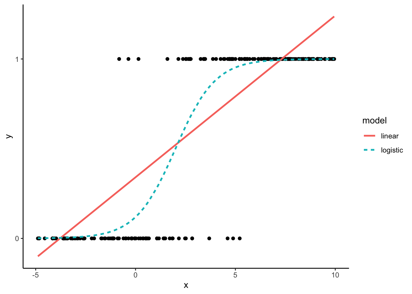
Logistic regression is a versatile and widely used statistical technique designed for modeling relationships between variables, particularly when the dependent variable represents binary outcomes. This methodology is particularly well-suited for scenarios where the outcome of interest is a binary event, such as whether a team wins or loses a match, whether a patient has a disease, or whether a customer makes a purchase. To visualise this, consider the plot below. This plot displays binary data, with responses being either 0’s or 1’s. Two models are fitted to the data (a linear and a logistic regression):

The linear regression model (depicted by the red line) operates under the assumption that the data is continuous, extending beyond the boundaries of 0 and 1. Conversely, the logistic regression model (indicated by the blue line) approaches 0 and 1 but never actually reaches them. This characteristic renders the logistic regression model more suitable for binary data.

The fundamental form of the logistic regression model is expressed as:

\[P(Y=1|X) = \frac{1}{1 + e^{-(\beta_{0} + \beta_{1}X_{1} + \beta_{2}X_{2} + \ldots + \beta_{n}X_{n})}}\]

where \(P(Y=1|X)\) represents the probability of the binary outcome \(Y\) being 1 given the predictors \(X_1, X_2, ..., X_n\), \(\beta_0\) is the intercept, \(\beta_1, \beta_2, ..., \beta_n\) are the coefficients associated with the independent variables \(X_1, X_2, ..., X_n\), and \(e\) denotes the base of the natural logarithm. The objective of logistic regression is to estimate the coefficients that maximize the likelihood of observing the given binary outcome data.

3 Assumptions

Logistic regression adheres to the following statistical assumptions:

Binary or Binomial Response: The response variable is either binary, representing two possible outcomes (e.g., success or failure, presence or absence), or binomial, representing the count of successes out of a fixed number of trials.
Independence: Each observation or case in the dataset is assumed to be independent of all other observations. This assumption ensures that there is no systematic relationship between the observations.
Linearity of Log-Odds: The relationship between the log-odds of the outcome variable and the predictor variable(s) is assumed to be linear. In other words, the logit function (log-odds) of the probability of the event occurring is a linear function of the predictors.
No Multicollinearity: There should be no multicollinearity among the predictor variables. Multicollinearity occurs when two or more predictor variables are highly correlated, which can lead to unstable estimates of the coefficients.

4 Case Study

4.1 What to expect

In this example we will re-examine the HansIll dataset (see Regression Modeling Strategies 2 - Poisson Regression for more details). We will use the variable Crit1and2 as our dependent variable. Crit1and2 is a binary variable that represents whether participants meet the criteria 1 and 2 of the Jackson’s common cold score (basically, do they show signs of having the common cold).

We will learn how to fit logistic regression models that contain both single and multiple predictors. We will also construct models that include interaction terms. Finally, we will use residual diagnostic tests to inspect the assumptions of our models.

4.2 Data Loading and Cleaning

First, we’ll load the HansIll dataset from the speedsR package into our R environment.

# Load the speedsR package
library(speedsR)

# Access and assign the dataset to a variable
Illness <- HansIll

4.3 Initial Exploratory Analyses

As always, it is good practice to explore our data descriptively, before we build our models. Much of this has already been covered in Exploratory Data Analysis (EDA) in Sport and Exercise Science, so we will only provide a short example here.

4.3.1 Data organisation

HansIll is a dataset that contains 39 variables. Some of the more relevant variables (to this exercise) are listed below:

ID: The participant’s ID number
group: The testing condition for the participant, 4x(8x40/20s), 4x(12x40/20s) or 4x8min
time: a binary factor to indicate results for either pre or post tests
Crit1and2: A binary (true / false) variable that displays whether participant meets criteria 1 AND 2 of the Jackson Common Cold score
vo2_rel: Relative VO2peak (L/min)

Note that for this lesson we will only be using the post-test measurements. As such we should create a filter to only include these measurements (i.e. when time is post). The code below has also renamed the Crit1and2 variable to Cold and changed the labels to ‘Yes’ and ‘No’:

Illness_post <- Illness |>
  filter(time == 'post') |>
  dplyr::select('group', 'Crit1and2', 'vo2_rel') |>
  rename(Cold = Crit1and2) |>
  mutate(Cold = factor(case_when(
    Cold == TRUE ~ 'Yes',
    Cold == FALSE ~ 'No'
  ))) |> 
  mutate_if(is.character, as.factor) |>
  
  # Also create a variable that codes Cold into 0s and 1s
  mutate(Cold1 = ifelse(Cold == 'Yes', 1, 0))

4.3.2 Summary statistics

We can use the skimr package to quickly obtain summary statistics for our chosen variables:

skimr::skim(Illness_post)

Data summary
Name	Illness_post
Number of rows	25
Number of columns	4
_______________________
Column type frequency:
factor	2
numeric	2
________________________
Group variables	None

Variable type: factor

skim_variable	n_missing	complete_rate	ordered	n_unique	top_counts
group	0	1	FALSE	3	4x(: 9, 4x(: 8, 4x8: 8
Cold	0	1	FALSE	2	No: 17, Yes: 8

Variable type: numeric

skim_variable	n_missing	complete_rate	mean	sd	p0	p25	p50	p75	p100	hist
vo2_rel	0	1	65.50	6.81	52.1	61.2	65.4	69.4	78.7	▂▇▇▅▃
Cold1	0	1	0.32	0.48	0.0	0.0	0.0	1.0	1.0	▇▁▁▁▃

We can use the table and prop.table functions to explore the Cold variable further:

table(Illness_post$Cold)


 No Yes 
 17   8

prop.table(mosaic::tally(~Illness_post$Cold))

Illness_post$Cold
  No  Yes 
0.68 0.32

Next, let us examine this Cold proportion over the group factor:

Illness_post |> 
  group_by(group) |> 
  count(Cold) |> 
  mutate(prop = n/sum(n)) |> 
  ggplot(aes(group, prop)) +
  geom_col(aes(fill = Cold)) +
  geom_text(aes(label = scales::percent(prop),
                y = prop,
                group = Cold),
            position = position_stack(vjust = 0.5))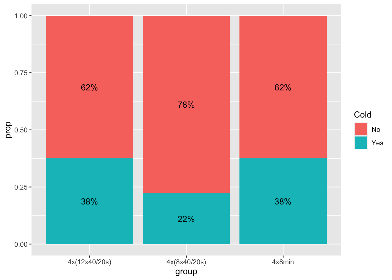

If we consider including a continuous term in our model (in this case: vo2_rel), the logit should be linearly related. We can investigate this assumption by constructing an empirical logit plot. In order to calculate empirical logits, we first divide our data by group. Within each group, we divide vo2_rel into subsets of equal sizes. Given the small size of this data set, we will use three groups:

Illness_post <- Illness_post %>%
  group_by(group) %>%
  mutate(cuts = cut_number(vo2_rel,3)) |> 
  ungroup()

Within each group, we calculate the proportion, \(\hat{p}\) that reported meeting the criteria for the common cold, and then the empirical log odds, \(log(\frac{\hat{p}}{1-\hat{p}})\), that a person meets this criteria:

emplogit1 <- Illness_post %>%
  group_by(group, cuts) %>%
  summarise(prop.Cold = mean(Cold1), 
            n = n(),
            midpoint = median(vo2_rel)) %>%
  mutate(prop.Cold = ifelse(prop.Cold==0, .01, prop.Cold),
         emplogit = log(prop.Cold / (1 - prop.Cold)))

Finally, we can plot this data:

ggplot(emplogit1, aes(x = midpoint, y = emplogit, color = group)) +
  geom_smooth(method = "lm", se=F)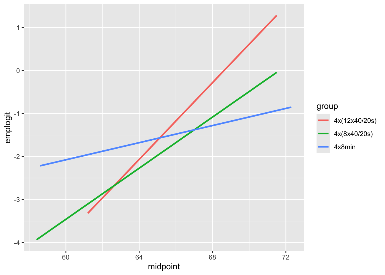

From this plot we can see that all three groups exhibit an increasing linear trend on the logit scale indicating that increasing vo2_rel is associated with a higher chance of having the cold and that modeling log odds as a linear function of vo2_rel is reasonable. The slopes between the three groups are not similar, so we should consider an interaction term between vo2_rel and group in the model.

4.4 Estimation and Inference

4.4.1 Continuous predictor

To begin, we will consider a simple model with only one predictor: vo2_rel. In R, we can use the glm() function, specifying the formula, family and data. For logistic regression, we will specify the family to be binomial.

model1 <- glm(Cold ~ vo2_rel,
    family = binomial,
    data = Illness_post)

We can then use the coef() function to obtain the coefficients:

coef(model1)

(Intercept)     vo2_rel 
-15.4722880   0.2202615

From this output, we can see that the intercept (\(\beta_{0}\)) and the coefficient for vo2_rel are -15.47 and 0.22, respectively. We can substitute these into the logistic regression equation (see Section 2) as follows:

\[P(Cold)=\frac{e^{\beta_{0}+\beta_1VO2_{rel}}}{1+e^{\beta_{0}+\beta_1VO2_{rel}}}\]

\[P(Cold)=\frac{e^{-15.47+0.22VO2_{rel}}}{1+e^{-15.47+0.22VO2_{rel}}}\]

We can interpret the coefficient on vo2_rel by exponentiating the coefficient value, \(e^{0.22}=1.25\) indicating that the odds of having a Cold increase by 25% for each additional increase in vo2_rel. We can also use the tab_model() function to quickly exponentiate the coefficients and confidence intervals:

sjPlot::tab_model(model1)

	Cold
Predictors	Odds Ratios	CI	p
(Intercept)	0.00	0.00 – 0.01	0.020
vo2 rel	1.25	1.06 – 1.58	0.025
Observations	25
R² Tjur	0.269

4.4.2 Categorical predictor

Suppose we wanted to build a model with the categorical variable, group. In R, this would be written as:

model2 <- glm(Cold ~ group,
    family = binomial,
    data = Illness_post)

And using the sjPlot package, we quickly obtain the exponentiated coefficients and confidence intervals:

sjPlot::tab_model(model2)

	Cold
Predictors	Odds Ratios	CI	p
(Intercept)	0.60	0.12 – 2.45	0.484
group [4x(8x40/20s)]	0.48	0.05 – 3.94	0.494
group [4x8min]	1.00	0.13 – 7.98	1.000
Observations	25
R² Tjur	0.025

We can interpret these results as:

The odds of having a cold are 52% lower for those in the 4x(8x40/20s) group compared to those in the 4x(12x40/20s) group, albeit this is not statistically significant.
The odds of having a cold are approximately the same for those in the 4x(4x8min) group compared to those in the 4x(12x40/20s) group, albeit this is not statistically significant.

Note that our sample size (n = 25) is quite small, so there is a possibility that we just don’t have the statistical power to detect these effects.

4.4.3 Multiple predictors

Similar to linear regression, we can construct our logistic regression models to include multiple predictors:

model3 <- glm(Cold ~ vo2_rel + group,
    family = binomial,
    data = Illness_post)

sjPlot::tab_model(model3)

	Cold
Predictors	Odds Ratios	CI	p
(Intercept)	0.00	0.00 – 0.01	0.024
vo2 rel	1.26	1.06 – 1.65	0.028
group [4x(8x40/20s)]	0.35	0.02 – 4.29	0.425
group [4x8min]	0.90	0.07 – 11.17	0.933
Observations	25
R² Tjur	0.290

We can interpret these results as:

The odds of having a Cold increase by 26% for each additional unit increase in vo2_rel (95% CI = 1.06 to 1.65, p = .028), when controlling for group.
The odds of having a cold are 65% lower for those in the 4x(8x40/20s) group compared to those in the 4x(12x40/20s) group, albeit this is not statistically significant, when controlling for vo2_rel.
The odds of having a cold are 10% lower for those in the 4x(4x8min) group compared to those in the 4x(12x40/20s) group, albeit this is not statistically significant, when controlling for vo2_rel.

4.4.4 Interaction Effects

Earlier, when we plotted the empirical logits for vo2_rel, for each cycling group, we observed a potential interaction effect. Thus, we can attempt to add an interaction term to our model:

model4 <- glm(Cold ~ vo2_rel + group + vo2_rel*group,
    family = binomial,
    data = Illness_post)

sjPlot::tab_model(model4)

	Cold
Predictors	Odds Ratios	CI	p
(Intercept)	0.00	NA – 0.00	0.313
vo2 rel	2.35	1.13 – NA	0.314
group [4x(8x40/20s)]	237836171748565581824.00	0.00 – NA	0.417
group [4x8min]	50044898614373277696.00	0.00 – NA	0.432
vo2 rel × group [4x(8x40/20s)]	0.49	NA – 1.17	0.406
vo2 rel × group [4x8min]	0.51	NA – 1.22	0.429
Observations	25
R² Tjur	0.360

In the displayed output, it’s evident that several odds ratios are reported with astronomical estimates, while some confidence intervals are marked as NA (not available). This phenomenon arises due to the limited size of our sample. Particularly, when we disaggregate the dependent variable across all levels of our main and interaction effects, the precision of estimates diminishes. Consequently, accurate determination of these estimates becomes challenging within the constraints of our dataset. Thus, we should revert back to model3, which did not include the interaction effect.

4.5 Evaluating our model

summary(model3)


Call:
glm(formula = Cold ~ vo2_rel + group, family = binomial, data = Illness_post)

Coefficients:
                  Estimate Std. Error z value Pr(>|z|)  
(Intercept)       -16.0594     7.1179  -2.256   0.0241 *
vo2_rel             0.2347     0.1065   2.204   0.0275 *
group4x(8x40/20s)  -1.0488     1.3147  -0.798   0.4250  
group4x8min        -0.1053     1.2491  -0.084   0.9328  
---
Signif. codes:  0 '***' 0.001 '**' 0.01 '*' 0.05 '.' 0.1 ' ' 1

(Dispersion parameter for binomial family taken to be 1)

    Null deviance: 31.343  on 24  degrees of freedom
Residual deviance: 22.875  on 21  degrees of freedom
AIC: 30.875

Number of Fisher Scoring iterations: 5

In Regression Modeling Strategies 1 - Linear Regression, we learnt how to use fit metrics such as R^2, BIC, RMSE, etc., to evaluate our model. For logistic regression, one approach is to use our model to compute the probability that each subject has the cold:

probabilities <- model3 %>% predict(Illness_post, type = "response")
head(probabilities)

        1         2         3         4         5         6 
0.1550538 0.6730356 0.4344277 0.8892623 0.1847837 0.4058471

In the output above (which shows the first 6 subjects), probabilities of having a cold were computed based upon subject’s vo2_rel measurements and cycling group allocation. For example, subject 1 only has a 15.5% chance, whereas subject 4 has an 88.9% chance, of having a cold based upon the model.

Using an arbitrary threshold (default: 0.50), we can classify the probabilities into 1 = ‘cold’ or 0 = ‘no cold’:

predicted.classes <- ifelse(probabilities > .5, 1, 0)

cbind(probabilities, predicted.classes) |> head()

  probabilities predicted.classes
1     0.1550538                 0
2     0.6730356                 1
3     0.4344277                 0
4     0.8892623                 1
5     0.1847837                 0
6     0.4058471                 0

From the output above (whih shows the first 6 subjects), we can see that using a threshold of 0.50, subject 2 (probability = 0.67) and subject 4 (probability = 0.89) would be predicted to be having a cold. From these 6 subjects, the remaining 4 subjects have probabilities less than the threshold of 0.50, therefore they would be predicted to be not having a cold.

Finally, we can compare these predicted classes to whether or not the subjects actually had a cold:

library(caret)
cm <- confusionMatrix(factor(predicted.classes, levels = c(1,0)), 
                factor(Illness_post$Cold1, levels = c(1, 0)))
cm$table

          Reference
Prediction  1  0
         1  3  2
         0  5 15

These results reveal that:

Of the 5 subjects predicted to have the cold, 3 of them did have the cold
Of the 20 subjects predicted to not have the cold, 15 of them did not have the cold

Based upon these figures, the overall accuracy of this model is 72%:

cm$overall[[1]]

[1] 0.72

Now, whilst this does seem like a reasonably high accuracy rating, there are some issues that we should consider:

We did not split the data into training and testing sets (see Lesson 1). Due to our small sample, splitting the data would make it very difficult to estimate the effects. This meant that we made predictions on the same data that was used to build the model. This likely would have resulted in overfitting the model, explaining the high accuracy rating.
We chose an arbitrary value of 0.50 for the threshold to predict classes. Choosing a threshold without considering the specific context or the costs associated with false positives and false negatives may not be optimal. Different threshold values could lead to varying trade-offs between sensitivity and specificity, which are important considerations in binary classification tasks. Methods such as Receiver Operating Characteristic (ROC) curve analysis to calculate Area Under the Curve (AUC) can help with this.

5 Conclusion and Reflection

In conclusion, this guide has provided an overview of regression modeling techniques suitable for binary variables, beginning with the assumptions underlying such models. We explored logistic regression models different types of predictors: continuous, categorical, continuous an categorical, and interactions. We learnt how to make predictions with our model to assess the accuracy of classification.

Throughout our discussion, we applied these regression techniques to a practical example of predicting whether or not someone has he cold, using two predictor variables. In our example we saw the limitations of a small data set, and it’s impact on interpretability. Nonetheless, this lesson provides a guide for you to be able to implement your own logistic regression models.

6 Knowledge Spot Check

Question 1
Solution

What type of outcome variable is typically used in logistic regression?

Continuous
Binary
Count
Ordinal

Binary

Logistic regression is commonly used for binary outcome variables, where the dependent variable has two possible outcomes, such as success/failure, yes/no, or presence/absence.

Question 2
Solution

What is the link function commonly used in logistic regression?

Identity function
Logit function
Exponential function
Log function

Logit function

The logit function, also known as the logistic or log-odds function, is the link function in logistic regression. It models the log-odds of the probability of the event occurring as a linear function of the predictor variables.

Question 3
Solution

In logistic regression, what does an odds ratio (OR) greater than 1 indicate?

The event is less likely to occur as the predictor variable increases.
The event probability decreases with the predictor variable.
The event is more likely to occur as the predictor variable increases.
There is no relationship between the predictor variable and the event probability.

The event is more likely to occur as the predictor variable increases.

An odds ratio greater than 1 indicates that the odds of the event occurring increase as the predictor variable increases, holding all other variables constant.

Question 4
Solution

What does the assumption of linearity in logistic regression refer to?

The predictors must have a linear relationship with the outcome variable.
The residuals of the model must be linear.
The outcome variable must be linearly distributed.
The predictors must have a linear relationship with the log-odds of the outcome variable.

The predictors must have a linear relationship with the log-odds of the outcome variable.

In logistic regression, the assumption of linearity pertains to the relationship between the predictor variables and the log-odds (logit) of the outcome, not the outcome variable itself.

Question 5
Solution

Which of the following best describes why multicollinearity is problematic in logistic regression?

It increases the model’s accuracy.
It makes it difficult to isolate the effect of individual predictors on the outcome.
It causes the outcome variable to be skewed.
It violates the assumption of binary outcomes.

It makes it difficult to isolate the effect of individual predictors on the outcome.

Multicollinearity arises when two or more predictor variables are highly correlated, leading to instability in coefficient estimates and making it difficult to determine the unique contribution of each variable.